
In the salary cap world, hockey is a game of resource allocation. Each team is given a set amount of money to acquire players. Consequently, hockey inevitably becomes about tradeoffs. When building a team, every dollar spent on one player is a dollar that can’t be used for another. There are certainly times when you can get a bargain, but you will always have to make decisions about spending priorities.
One frequent prioritization question is high-end quality vs. depth. How much should a team focus on the very top of its lineup vs. ensuring it has adequate depth? Should a team maximize its strengths or minimize its weaknesses?
This question is relevant to many front office decisions. The Bruins traded Tyler Seguin for several assets, and some argued that the Penguins should do the same with Evgeni Malkin to improve their depth. As Steven Stamkos approached free agency, many teams were deciding just how much they would be willing to pay him while knowing that signing him would inevitably come at a cost lower down the roster.
We can think through these tradeoffs by studying talent distribution within a team. If you hold total talent constant, is it better to have a team where everyone is equally talented, or one where a few elite players are trying to shelter a few terrible ones? We know from current Florida Panthers consultant Moneypuck that contending teams have at least one elite player, but to my knowledge, very little work has been done on the broader question of total team structure. This article mirrors my presentation at the Vancouver Hockey Analytics Conference 2017, at which I dug into talent inequality within teams to demonstrate:
- Hockey is a strong link game, i.e., the team with the best player usually wins
- Therefore, teams should prioritize acquiring the very best elite talent, even at the cost of having weaker depth than opponents
- This is important for roster construction now and has the potential to become even more important as teams get better at assessing talent and market inefficiencies become less common
This article has three parts. First, I introduce the concept of strong link and weak link games, which provides theoretical backing to the topic. Second, I adapt work from soccer to assess whether the best or worst player on the team is more important to success, and show it is the best player. Finally, I apply economic measures of resource distribution to demonstrate that teams with talent inequality do better than balanced ones.
The Legend of Zelda Link: Defining Strong and Weak Link Games
I first became familiar with the concept of strong and weak games in The Numbers Game, a book by Chris Anderson and David Sally on soccer analytics. In it, they define a strong link game as one where the team with the best player usually wins. In contrast, in a weak link game, the team without the worst player usually wins.
Anderson and Sally demonstrate that soccer is a weak link game: upgrading the weakest player on a team does more for success than upgrading the best player by an equal amount. This has huge implications: owners of soccer teams may be signing star players to record-breaking contracts, but if their only goal is to win, they would be better served by foregoing the star-power and investing in depth.
One can see intuitively what makes soccer a weak link game. It’s a low scoring game, so mistakes can matter a lot. In addition, each player has possession for a small fraction of the game. Lionel Messi is capable of doing incredible things once he has the ball, but he can’t get it until his teammates complete several passes. One weak link in the middle of the field can prevent Messi from ever seeing the ball.
In contrast, basketball is a strong link game. There are few players on the court at once, and one player can easily get possession. If Steph Curry or Lebron James wants the basketball and their team has possession, they will get it. That’s why the teams with these star players are almost always the ones making deep playoff runs.
Hockey does not easily fall into either of these categories. Like soccer, total scoring is low, and each player only has possession for small portions of the game. Furthermore, the best players are only on the ice for half the game, at most. On the other hand, like basketball, few players are on the ice at once, so an individual great player could have a large impact. In addition, because ice time is spread among so many players, the weakest links could be given very little ice time.
To demonstrate that hockey is a strong link game like basketball, we’ll need to dig into the analysis that Anderson and Sally put together for soccer.
Kings of Strong Style: The Importance of Elite Talent
Anderson and Sally demonstrate that soccer is a weak link game by focusing on the best and worst player on each soccer team. They run regressions to show that having a better weak link has a larger effect on total season points than having a better strong link. In this section, I’ll duplicate this work for hockey and come to the opposite conclusion: hockey is a strong link game, where the best player on the team is more significant to winning than the worst.
To determine the best and worst player on each team, I use DTMAboutHeart’s WAR measure. Obviously, it isn’t a perfect representation of all skater knowledge in the world, but for this analysis, it is a useful proxy for each player’s talent.
My dataset is each team from each season from 2008 – 2009 to 2015 – 2016. I transformed WAR into a rate stat based on TOI and made it a value between 0 and 1, based on its percentage value compared to the highest WAR in the dataset (Crosby 2013-2014). I then ranked the skaters (goalies excluded) on each team by their WAR that season; the player in first was labeled the strong link, and the player in 18th was the weak link. (Due to TOI restrictions, a few teams did not have 18 players with useable WAR measures. Rerunning this analysis with the 16th best skater reduces the missing values and shows similar results.) Here’s the relationship between the strong and weak link on each team:
The talent level of the team’s best player has no relationship to the talent level of the team’s worst player. This suggests that the tradeoffs I described at the beginning of this post are not so airtight that they are always necessary; some teams have managed to have both an elite best player and good enough depth that their worst player is okay. But which one impacts winning? Let’s look at their relationship with the team’s points that season:

Here are the first signs that hockey is a strong link game: whether the worst player on the team is good or bad has no correlation with how many points the team gets that season (correlation = -0.04). On the other hand, the best player’s WAR is correlated with season points (correlation = 0.348). The results are similar when replacing season points with goal differential.
Next, I applied Anderson and Sally’s methods by regressing the strong and weak link’s WAR on the team’s points. I also included the team’s total WAR since we know from Moneypuck that total team WAR is associated with team success. Results without the extra coefficient are similar. The formula is as follows:
Y = β0 + β1X1 + β2X2 + β3X3 + ε
Where Y is the team’s total points, X1 is the strong link’s WAR, X2 is the weak link’s WAR, X3 is the team’s total WAR, and ε is an error term.
The results: The F-statistic is significant and the adjusted R-squared value is 0.14, so we know this model is telling us something about how to acquire points, though there’s clearly a lot missing from it. Unsurprisingly, total WAR is significant. The strong link’s WAR is also significant, but the weak link is not. This demonstrates that hockey is a strong link game. Improving your best player has a bigger impact on winning than improving your worst player by an equal amount.
Gini as Tonic: Full Roster Talent Distribution
The above findings are interesting but limited. A team has more than 2 players, and the other ones matter. Ideally, we would expand on Anderson and Sally’s methods to incorporate how talent is distributed throughout the entire roster.
If we abstract the question to one of resource allocation between individuals (here the resource is talent), there are measures from other fields readily available. My background is in economics and business, where there are plenty of ways to measure how a resource is spread. Statistics – the field in which I continue to dabble – has several more. We can take these to measure talent inequality within teams.
I tried four different measures of resource talent distribution. From economics, I used the Gini coefficient, which measures income or wealth inequality within and between countries. Here, the equivalent of a highly unequal country is a team where a few players are incredibly talented while the bottom of the roster is awful. The Gini coefficient is a single number between 0 and 1 that measures this inequality. The Gini coefficient has been used in sports analytics before (see here and here), but typically as a measure of competitive balance between teams (and not without pitfalls)
Second, I use the Herfindahl-Hirschman Index, which is a business measure of how concentrated a market is. A team of Sidney Crosby plus ECHLers would basically be a talent monopoly, while a team with 20 exactly equal players would be a much more crowded, competitive market. Third and fourth, I use two common statistics measures: standard deviation and range. Like Gini, these metrics have been used to measure competitive balance across teams in the NHL (see Preissing and Fenn)
I took each of the four metrics individually and regressed them and total WAR on team points. The results were basically the same for all four. In each case, both total WAR and the measure of inequality were significant. More importantly, each regression showed that teams did better if they had highly unequal distributions of talent within their team.
Conclusion
Hockey is a strong link game. Getting the very best players is essential to success. Phrased this way, it sounds obvious. But the above shows that this is the case even at the cost of creating weaknesses elsewhere in the lineup. This has implications for many of the major decisions that general managers make.
When trading, this work suggests that quality is more important than quantity.* Tyler Seguin was traded for multiple pieces and Evgeni Malkin was rumored in plans to do the same, and I think that both Dallas and Pittsburgh are happy to have the best player rather than several lesser players. In free agency, it is better to spend cap space on a single star than on multiple pieces of the bench. For the draft, this piece provides rigorous evidence supporting the belief that tanking works, since tanking is one of the best ways to acquire elite talent (once again, see Moneypuck). Finally, I’d argue that this has implications for coaching as well: hockey is about creating goals, not avoiding mistakes, and there is a compelling case to give top players the freedom to make plays and win games.
These findings also nicely complement DTMAboutHeart’s RITHAC presentation, in which he suggested it is better to spread out top players on different lines rather than putting them together. That suggests that individual matchups are also strong link games, and it is best to have as strong a player as possible on the ice at all times.
These findings also matter when taking a step back and looking at the creation of a complete roster. If you’ll allow a bit of speculation, these results have made me think a lot about the Carolina Hurricanes. They have made a lot of smart moves and have strong contributors throughout their lineup. However, they have yet to find consistent success. They have good players, but I don’t think that many people would argue that they have a top-10 player in the league. As they determine their next moves, perhaps it is necessary to sacrifice some of their current strengths in pursuit of game-changing talent.
There are numerous ways that this work can be improved. First, it would certainly benefit from attention from a real statistician. I have tried my best to be rigorous and transparent, but my statistics knowledge is limited and it is possible that this work is flawed.
Assuming the general conclusions are right, more work on the effect size of roster imbalances would help define exactly how much the tradeoff for elite talent is worth. Second, Jack Han suggested splitting this work into offense and defense to see if the weak link / strong link distinction is clearer in one side of the game, and this sounds like a worthwhile investigation. In addition, it would be nice to find a compelling method for including goalies in this analysis. Finally, more work should be done to better understand the marginal cost of improving each part of the roster.
All of the data and code used for this work, as well as my slides from VANHAC are available here.
Thank you to Dom Luszczyszyn, Micah Blake McCurdy, and Dawson Sprigings for data collection help
*sorry for ruining your trade proposals, HFBoards

Hi Alex,
Awesome work. Is it possible for you to publish the dataset you’re using here, for reproducibility?
Thanks
Thank you! The data should all be available in the dropbox link at the bottom of the post (I’ve also copied it below). If that isn’t working or some of the data is missing, let me know and I’ll update it
https://www.dropbox.com/sh/0evs81yi58kduny/AABw3y5CPDOmQd4OHVGGnjNha?dl=0
Ugh… My fault for not reading properly! Thank you very much. I hope you continue the great work.
“X1 is the strong link’s WAR, X2 is the weak link’s WAR, X3 is the team’s total WAR,”
Wondering if the variables are independent of and uncorrelated with each other.
Given that X3 is clearly a function of X1 and X2 (among other things), they’re definitely not independent. But as you say, we’re actually interested in whether they’re correlated or not, and intuitively, I would think that they would be. Specifically, I would think X1 and X3 are correlated, since great players make up a significant portion of their team’s WAR, whereas the spread is much smaller for worse players.
Is this a problem for the regression?
Potentially, yes. Generally speaking, correlation among predictors can cause the regression to break down entirely because there will be no unique solution for the parameters (due to the underlying linear algebra). That didn’t happen here. However, in general, it would make our estimates of the predictors less precise, and their standard errors larger. It doesn’t really change the overall fit, however.
Thanks, Arvind! As you’ve already discussed, yes, X1 and X3 are correlated while X2 is not correlated with either. This is one reason why I don’t trust reading too much into the effect sizes. As you mentioned, I don’t think the collinearity effects the main conclusions, but I’m open to new info.
A few questions for my own edification:
(1) Is independence an issue separate from the collinearity issue?
(2) Collinearity seems like a foundational issue, so I was wondering if your reply ought to be dealt with in the Main body of the text–perhaps as a potential methodological problem–and at greater length than can be given in the Comments Section. Thanks for the discussion.
(1) I think there are nuances between the two, but in this case they’re pretty similar
(2) Potentially, sure. I’m always balancing the hockey and the graphs in Hockey Graphs, and it’s tough to know how much detail to cover in the statistics without boring a more general audience. Since the audience here tends to be primarily hockey fans first and statisticians second, my approach has generally been to explain the stats approach at a high level and what it means for the results, then provide all of the code for people who want to take a deeper look (especially since I don’t have the knowledge base to be a particularly good stats teacher). In fact, the feedback on this post I’ve received has been more from people who couldn’t follow the math than people looking for more.
(3) I guess I don’t entirely understand the issue. My (inadequate) understanding, at a high level of generality:
We’re trying to figure out the particular effects of independent variables using multiple regression. Here, the particular effects in terms of Total Points. The independent variables are Strong WAR, Weak WAR, and Total WAR. Strong WAR and Total WAR are admittedly correlated (and it seems to me that Weak WAR will be correlated with Total WAR as well, how could it not?). There’s also the Error Term. So if there’s all this correlation among independent variables, as well as error, how can the regression provide adequate assurance that we are getting at the particular effects of Strong WAR and not, e.g., Total WAR (not sure if/how error term adds complexity here)? In particular, how does it provide us with the rational basis to conclude:
“Unsurprisingly, total WAR is significant. The strong link’s WAR is also significant, but the weak link is not. This demonstrates that hockey is a strong link game. Improving your best player has a bigger impact on winning than improving your worst player by an equal amount.”
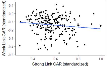
It turns out that weak WAR is so small and the result of so many other factors, it’s independent of total war. The 2nd image in this post is the best illustration of that
As to your main point, those concerns would definitely come into play in some ways. They’re why I didn’t try to interpret the effect sizes, for example: the exact coefficients for strong WAR and total WAR aren’t trustworthy. It also reduces the power of the model, so there was a chance that it would fail to predict total points even if a relationship existed. However, the correlation doesn’t mess with the overall predictivity of the model, and in this case, adding strong war does improve that predictivity*. That’s why I feel comfortable that strong WAR, despite its relationship with total WAR, is adding additional information and that increasing it also increases points.
(*This claim would be strengthened with better out-of-sample testing. I’ve done some of that on my own, but haven’t cleaned up and shared the code.The dropbox link does have everything so that people can do it on their own.)
One thing to think about: in hockey strong players tend to be matched against strong players, (though that is not always the case).
In ascertaining the impact of weak links on winning and losing, it’s important to consider a weak link relative to his general level of competition. It may be easier to hide three or four weak players in hockey by playing them little or only against other weaker players. But if you have a weak link in your Top 6 forwards or one or two weak links in your Top 4 defence, they may not be terrible players, and almost certainly won’t be the worst players on their team, but they will nonetheless cause a major amount of damage because of the gap between them and the competition they face, the gap between them and other players in that same role around the league. In this way, hockey can be seen as a weak link game.
If you have a weak link in net, a weak link in your Top 4 d, or a weak link in your top 4 or 5 forwards, that’s where you lose the game.
Of course, a super strong situation in that same Top 4 dmen or Top 5 forwards creates the same imbalance.
Overall, lack of possession time, low scoring, and harm caused by weak links vs tough comp, I lean to hockey being weak link game.
Hi David, thanks for sharing. That’s an interesting concept – almost a “weak link out of those players who can’t be protected by tactics”, assuming I understand correctly.
I wonder how much the strong link benefits from the opposite side of the matchups you described. If McDavid gets a couple of shifts against a #6 D, he can probably blow by him. Does he benefit from this mismatch disproportionately more than an average typical first-line forward? I don’t know.
I’d love to dig into the tactics side of this some more; sort of a micro-level view of strong/weak link. One way would be to look at the shift level: determine the strong and weak links on the ice at every time and see how well their team does. Unfortunately, I haven’t done it because assigning the links at that level (out of just the 10 skates on the ice) pushes WAR a bit further than I’m comfortable. As our WAR metrics get better, or if somebody thinks of a better methodology, it would be a very interesting view. It would really help validate how matching happens and how well it goes for each team.
Would be curious to see what the impact of a strong link vs. 3 (or more) weak links is, too. When you trade away a game changing player, you get a full bottom 6 line. Does Crosby matter more to the Penguins than whoever their 4th line centre is? Obviously. Does having an entire 4th line that’s way better than the standard 4th line in the league matter less than Crosby vs the average top line centre? That’s a different question, and I’d argue it’s more of a representative one, since upgrading the strong link is probably similar in cost to upgrade 3 (or in some cases maybe 5) weak links.
On a one to one basis I absolutely agree that the best player drives the team more than the worst player sinks it. But does $10,000,000 drive the team more in one player or across 4?
“Why not just do both?” – Steve Yzerman
Hi Alex.
Nice work. Curious if you would consider salary instead of WAR as a proxy for value? Think of a team as a series of investments, a portfolio of equities if you will.
Some teams will invest in high quality, high growth tech companies and others will focus on those toward the bottom of the Fortune 1000 but have good “measureables”.
Maybe the salary committed to each line as a percentage of total team expenditures can get to your strong link- weak link argument a different way?
Thanks!