
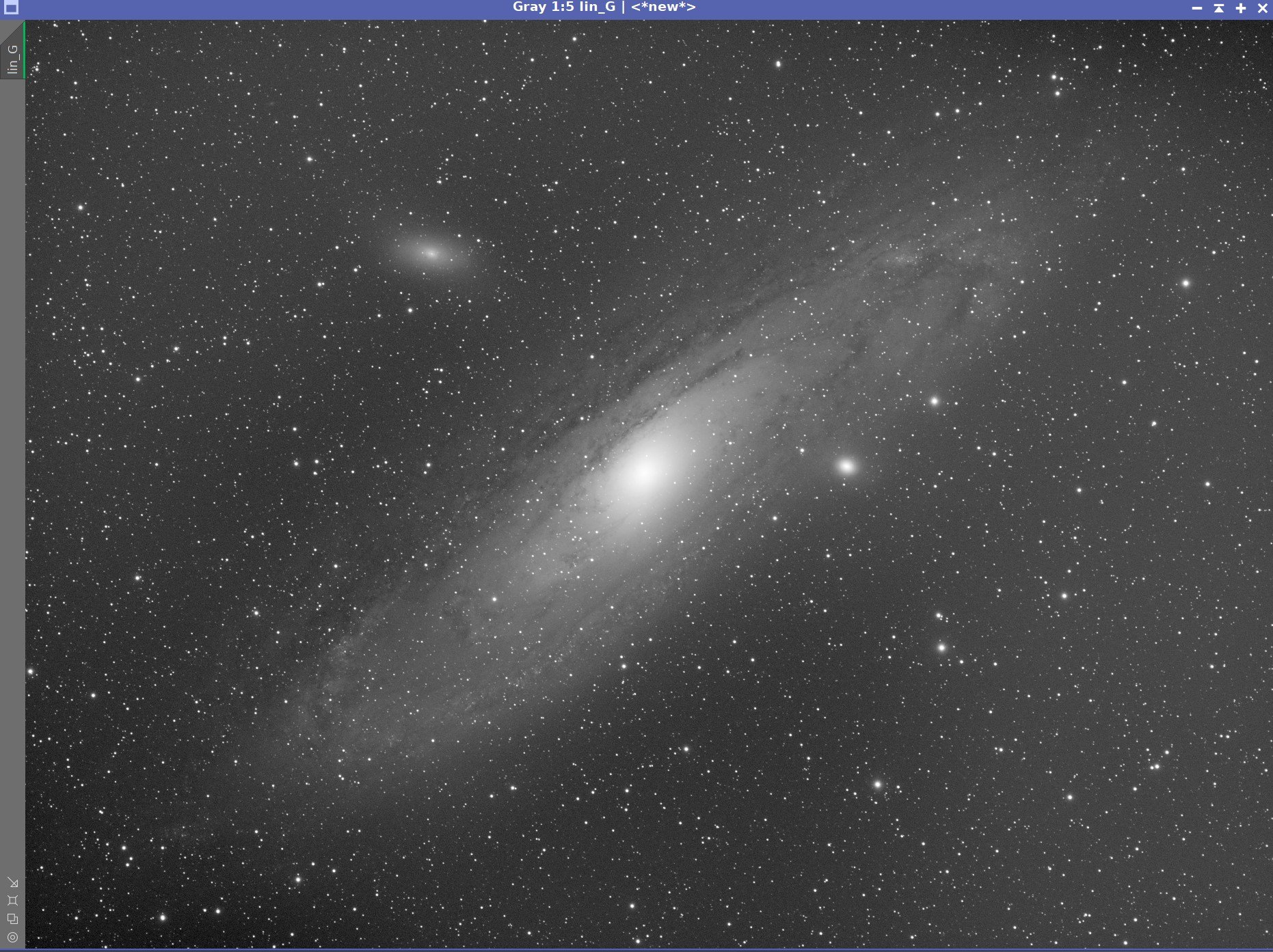
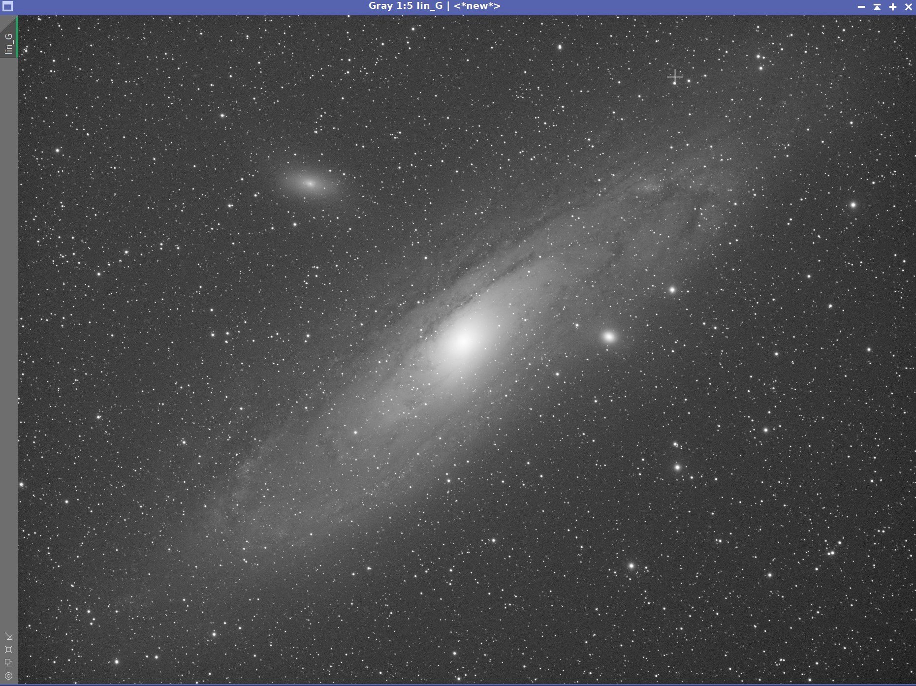
Messier 31 - The Andromeda Galaxy in LHaRGB - 6 hours
Date: November 24, 2021
Cosgrove’s Cosmos Catalog ➤#0088

Messier 31 - The Great Andromeda Galaxy (Click image for full resolution version via Astrobin.com)
October 2022 - Named as “Picture of the Month” by the Webb Deepsky Society on their website!
(Click to enlarge)
Table of Contents Show (Click on lines to navigate)
About the Target
Messier 31 is one of the brightest jewels in the night sky. This is my third attempt at this object. Rather than compose a brand new summary for this post, I will simply quote my description from a previous one:
"Messier 31 is also known as NGC 224 and the Andromeda Galaxy, or as the Andromeda Nebula before we knew what galaxies were. It can be seen by the naked eye in the constellation Andromeda (how appropriate!) and is our closest galactic neighbor located 2.5 Million light-years away. It is estimated that it contains about one trillion stars - twice that of our own Milky Way.
M32 (at the top left closest to the core of M31) and M110 (at the bottom right)can be seen in the frame. These galaxies are neighbors and are, or have been, interacting with M31. M32 appears to have had a close encounter with M31 in the past and it is believed that M32 was once much larger and M31 stripped away some of that mass and triggered a period of extensive star formation in M32's core that we see the result of today. M110 is also currently interacting with M31 now.
As I shared with my first image of M31 taken about a year ago, it is projected that Our Milky Way and M31 will collide in the future, forming an elliptical galaxy. Don't sweat it - it won't happen for 4.5 billion years from now…"
Annotated Image

This Annotated Image of M31 was created using the ImageSolver and Annotate Image Scripts in Pixinsight.
Location in the Sky

IAU/Sky & Telescope Constellation Chart with Messier 31 indicated by a yellow arrow.
About the Project
The Andromeda Galaxy is one of the most photographed objects in Astrophotography.
I have already shot it two times. Everybody who wishes to try astrophotography, or claims to be an Astrophotographer, has shot and posted images of this object.
Frankly - it is almost cliché.
So why bother? Why add to the enormous trove of already existing images?
Well - for one thing - it is very big and very bright.
It measures some 1 x 3 degrees. The full moon measures 0.5 degrees, so M31 is 2 moons by 6 moons in size. This surprises most people.
It has an apparent magnitude of 3.5 - is one of the farthest objects that can be seen with the naked eye.
When you are talking about a distance of 2.5 Million light-years - you are dealing with scales that your mind has trouble comprehending. When you see M31 with your naked eye, think of it - you are responding to a sensation caused by photons that had traveled for 2.5 million years before they landed on your retina!
Short and crude exposures will show amazing details - the bright core, the spiral arms, companion galaxies, dust lanes, knots, and twists of matter. M31 is a feast for the eyes.
So why make yet another image? What not? It's simply an amazing target with many opportunities to put your stamp on it and see what you can do!
When I first started, I was getting some early results - and more than a little impressed with myself. Of course, I was probably the only person in the world who was impressed with what I had done. Then I took a short integration of M31 and did some simple processing - the results stunned me - it was just so impressive compared to my earlier images.
As I showed the image around to family and friends, they seemed impressed as well! “Wow! Did you take this?" While that kind of response was a little insulting, I was still very glad to finally be evoking in others some kind of positive reaction.
Previous Attempts
That first attempt with M31 can be seen HERE. My second attempt can be seen HERE.
I'll include the images below:
My first attempt at M31 - centered on the core of the galaxy - Sept 2019 (click to enlarge)
My second attempt Aug 2020 - this time I attempted to include the companion galaxies, M32 and M110. (Click to enlarge)
Both of these images were taken with my William Optics FLT 132MM APO Refractor with a focal length of 920mm. With this scope, I could not get the whole galaxy in the frame!
The William Optics 132mm FLT APO platform took my first two images of M31.

The Askar FRA400 Platform was used to shoot the new M31 image.
At the time, an OSC (One-Shot-Color) camera was used. It did a good job but did not have the flexibility of a mono camera with wideband and narrowband filters.
Now that I am getting good results with my wide field-portable FRA400 scope, I finally had the ability to get the whole galaxy in the field of view for the very first time - and I could also shoot with a mono camera.
My plan was to collect LRGB filter data along with some Ha subs. The Ha filter emphasizes areas of HII activity - typically associated with new star formation - and folds that into the image of the galaxy. When I have done this with other galaxies, I have been impressed with the drama it seems to bring to the image. Now with a large and detailed object like M31, it could be the icing on the cake.
So why shoot it again?
To see if I could better my earlier efforts.
To finally get a chance to get the whole galaxy into the image
To see what I could do by adding Ha data into the mix
To use more advanced processing techniques on it
To visit an old friend…
Data Capture
Between November 5th and 8th, we had a surprisingly good stretch of clear skies without the moon. As I have noted in my recent image project posts - this is a wonderful time of year if you have some decent weather since it gets dark early, and you can have as much as 12 hours of capture time each night. I still have to wait for my targets to clear the tree line - and I can only collect subs for a fairly short time before it again descends back into the trees. But I can capture targets one-after-another all night long!
In the end, I ended up with slightly over 6 hours of data. I had LRGB subs that were shot at 90 seconds each. I often shoot RGB subs with 120 seconds, but since the FRA400 astrograph is a faster f/5.5 optical system (compared to my other scopes with are f/7 and F/8.35, respectively), I opted for a shorter time.
Processing
While detailed processing notes are included below, I wanted to talk about some issues with this image.
First, I had to decide if I wanted to drizzle process this data or not. The camera/scope combination is slightly undersampled - which can produce squarish stars on a small scale. Drizzle processing avoids this by resampling the data cleverly and restoring some lost resolution. The downside is that images have 4X as many pixels - leading to really large image sizes. This means more disk space, more i/o, longer processing times, and in some cases - no longer allows you to use some techniques. But the quality can be great. For this image, I decided to drizzle process the data.
Second off, I had to decide how I wanted to add the Ha data into the image. There are several ways and techniques. In this case, I decided to add the Ha data to the red channel as part of creating my first color image.
To begin with, I processed my Ha, R, G, and B Master linear images in pretty much the same way. They had a common crop applied, and then I used DBE to remove gradients.
To create the color image, I used the SHO-AIP script to blend the four images into one RGB image - which in this case, was a HaRGB image. The SHO-AIP script allows you to add wideband and narrowband images and then specify how they are blended to create the color image. It also allows to prototype the look for a given blend and to experiment with different mix levels.
Once I had my HaRGB image, I ran DBE again to remove any color gradients and then used PCC to color calibrate the image. Finally, I ran the EZ-Denoise script to "knock the fizz" off the resulting linear image.
The Lum image had a separate processing path. It, too, had the same common crop applied. Then DBE was applied to remove gradients. Next, deconvolution was applied, followed by EZ-Denoise and a little MLT sharpening.
Finally, it was time to go nonlinear. MaskedStretch was used to do the first stretch for the HaRGB and the Lum image.
The color image was then stretched some more using the ArcsinhStretch tool - this stretches the image and preserves the high-end of the tone scale. This causes colors to look a bit more intense than they might normally look - but this is a good thing to do before adding the Lum channel into the image. Colors tend to wash out when they get above code values of 0.8. If they are already high, adding the lum data will push things higher, and colors can be watered down. The ArcsinhStretch script caused colors to have lower code values which will look great when the Lum data is folded in.
Finally, I used the LRGBComposition tool to fold in the Lum data. After some more tweaking, I was quite happy with the image, but I noticed that something was weird - the right side of the galaxy seemed to have a red balance, with almost no blue outer fringe, and the left side had a cool balance. It’s almost like the image was split down the center, and each side had a different color balance.
My initial image version had red color balance on the right side and a blue balance on the left (click to enlarge)
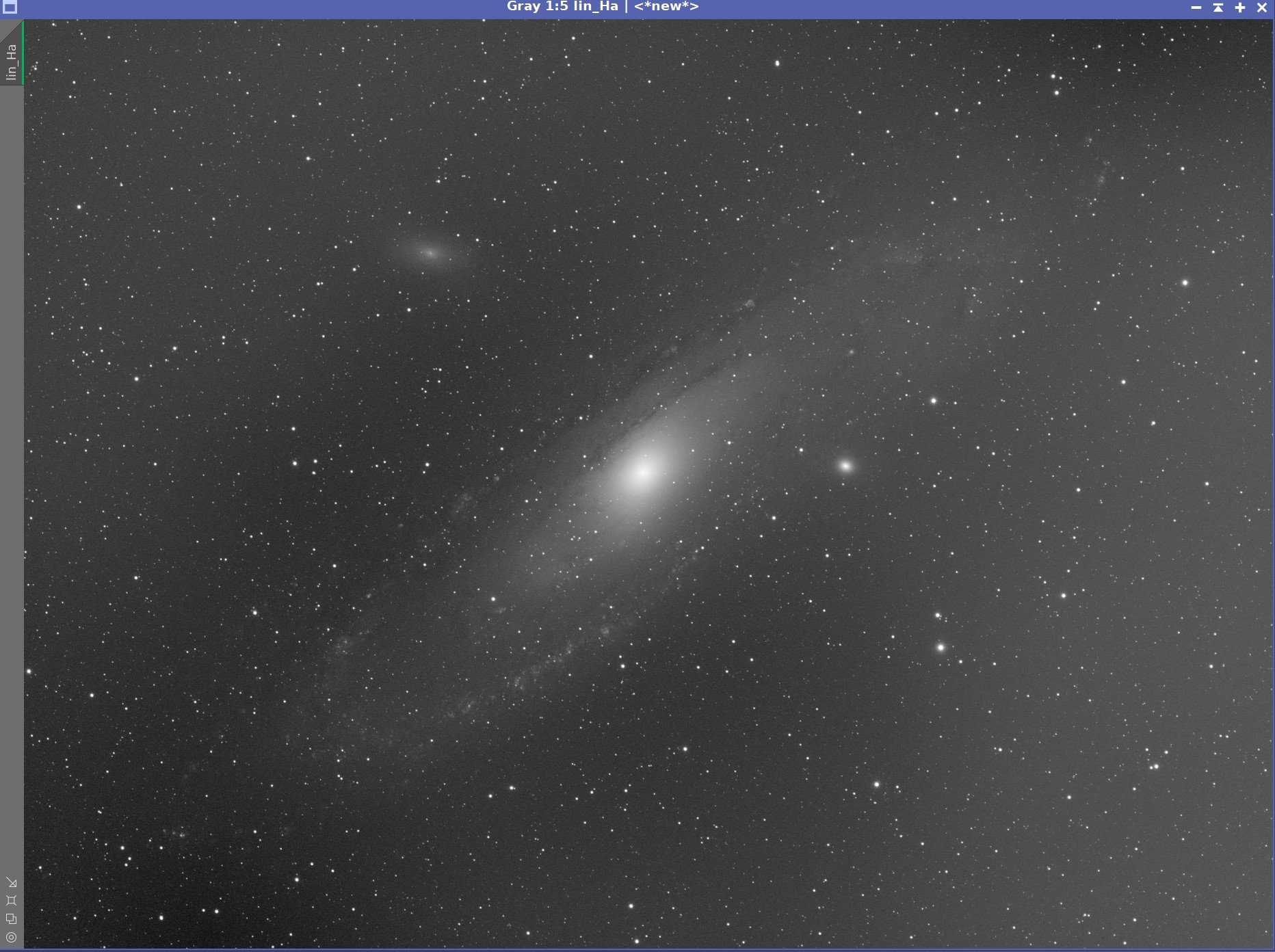
This seems to be caused by the Ha image. As you can see below, one side has knots and a prominent Ha glow, and the other side is defused with relatively little detail. This then caused a bias on one side and not the other.
Here is the linear Ha image. Note the ring of H2 “knots” and haze on one side the lack of detail on the other side (click to enlarge)
I thought this looked odd, so I created some partial Ha masks and adjusted the red side to better match the color balance of the left side. Here is the result:
The first attempt to balance the image by reducing the red balance on the right side of he image (click to enlarge)
The second version balanced out the image by adding red into the left side of the image (click to enlarge)
The image looks better with the color balanced consistently on each side in this version, but I thought the loss of the red balance reduced the overall impact of the image.
So I decided to try another approach.
This time I created a mask of the left side of the image and added more red to better match the right side. Then I matched the blue outer fringes on each side to get better color consistency. I was much happier with this version of the image, and this was the approach I used for the final image.
Why was the Ha different on one side of the galaxy compared to the other? To be completely honest - I have no idea. The data was what the data was!
Image Processing Detail (Note this is all mostly based on Pixinsight)
1. Assess all captures with Blink
Light images
Lum images - 4 images rejected due to heavy clouds
Red images - some very light gradients seen - but none removed
Green Images - some very minor gradients seen - but none removed
Blue Images - all frames look great!
Ha Images - clouds moved through - 5 images removed
Flat Frames - look great!
Flat Darks
Taken from IC1805 project. Greens are missing but have the same exposure time as red, so we can use those
Darks - taken from IC1805 project
2. WBPP Script
All images loaded into WBPP
Cosmetic correction enabled
Drizzle integration was chosen to deal with slight undersampling
Pedastal image of 50 used on Ha channel
Integration was enabled, and this simplifies DrizzleIntegration

WBPP setup

Post Processing View of WBPP
3. DrizzleIntegration
Default paramters used
Run for each image to create all image masters.
4. Dynamic Crop
A common best crop position was used and implemented with DynamicCrop
5. Dynamic Background Extraction
A custom sampling pattern created using Lum image
DBE with subtraction was used to remove gradients for all images.
Ha still showed some residual gradients, so the sampling pattern was adjusted and DBE run a second time.
Images below show before and after treatment with DBE.

Example of the sampling pattern used in DBE for all images

Lum before DBE

Red before DBE
Green before DBE

Blue before DBE
Ha before DBE

Lum After BDE

Red After DBE
Green After DBE

Blue After DBE

Ha After DBE
6. Create a Linear Color Image
Create Hargb image with SHO-AIP script
Experiment with 3 Variations
R = 50% R + 50% Ha
R = 25% R + 75% Ha
R= 75% R + 25% Ha
The 75% Ha variation was judged to be best.
Run DBE to get rid of any new color gradients.
25% weight on Ha

50% Weight on Ha

75% Weight on Ha

REsulting images. The Last one was best. These images are shown before DBE removed color gradients.
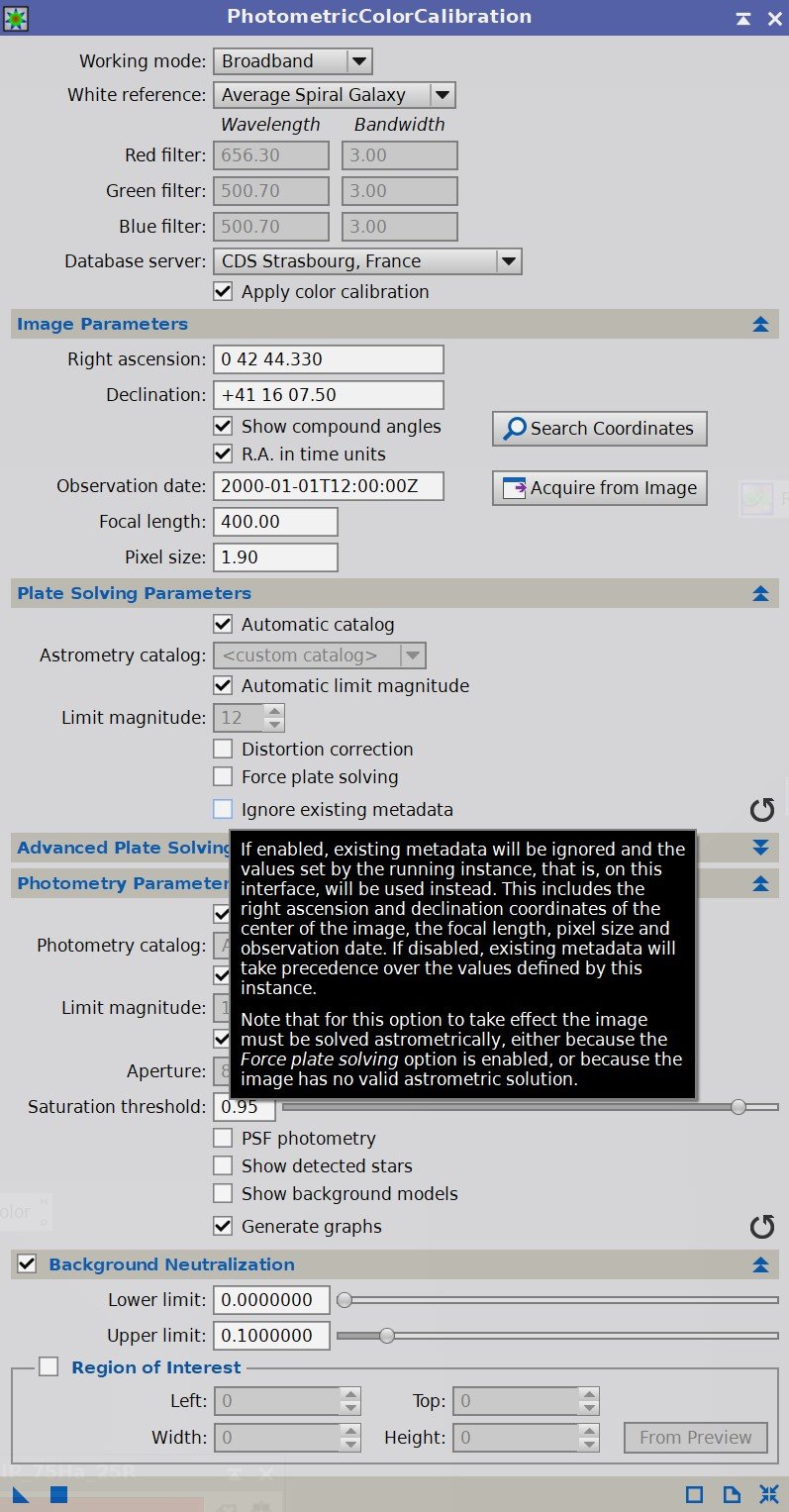
7. Color Calibration
Run PCC
set to half normal pixel size - 1.9 (because of drizzle processing)
grab m31 coordinates
Run


The color corrected HaRGB image
8. Run EZ-denoise on Color Image
Use defaults
HaRGB before EZ-Denoise (click to enlarge)
HaRGB after the Denoise operation (click to enlarge)
9. Go Nonlinear with the HaRGB Color Image
Select preview of a background area
Run MaskedStretch with the preview selected
Run ArcsinhStretch with a factor of 1.29 black threshold of 0.058. This finalizes the stretch and protects the color highlights.
HaRGB after MaskedStertch (Click to enlarge)

The ArcsinhStretch Panel Settings used.
HaRGB image after ArcSinhStretch (Click to enlarge)
10. Run Deconvolution on the Lum image
Create the Object Mask
create a copy of the Lum image, rename it.
Go nonlinear using the STF->HT method
Use HT to emphasize nebula and stars and suppress background
Create psf with PSFImage script
Create Local Support image
run Starmask
Scale: 6
Smoothness: 10
Check Aggregate
Check Binarize

Object Mask for the Lum image

Local Protection Image for Lum
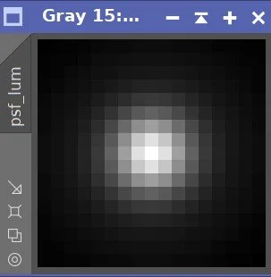
PSF for the Lum Image
11. Apply Deconvolution to the Lum Image
Apply Object mask to Lum Image
Setup Deconvolution tool to use the psf and local protection images
Select 3 previews
Test and Optimize the Global Dark Parameter with previews
Final - global dark 0.02 20 interactions
A section of the Lum image before Deconvolution (click to enlarge)
A section of the Lum image after Deconvolution i applied. Note the restored sharpness of the dust lanes and reduction of star size (click to enlarge)
12. Apply Noise Reduction to the Lum Image
We wish to preserve details since the Lum layer will provide most of that high-frequency information
Try doing noise reduction with two methods: EZ-Denoise (default params) and MLT (Standard Linear NR setup).
EZ-Denoise was seen as the better of the two results.
Starting noise level on the Lum image.
The results of MTL used in standard Linear NR mode.
The results from the EZ-Denoise script. This was the superior result and was used to move forward.
13. Go nonlinear with the Lum Image
Select a preview area with a good background sample
Select this with the MaskedStretch process and apply it to the Lum image
Use CT to boost tone scale with a slight “S” curve
Enhance smaller structures in Lum Image - Apply LHE with a radius of 122, a contrast limit of contrast 2.0, and the amount set to 0.2
14. Add Lum image to the HaRGB Image
Use LRCGCCombination with the nonlin_Lum image, and apply it to the HaRGB nonlin image
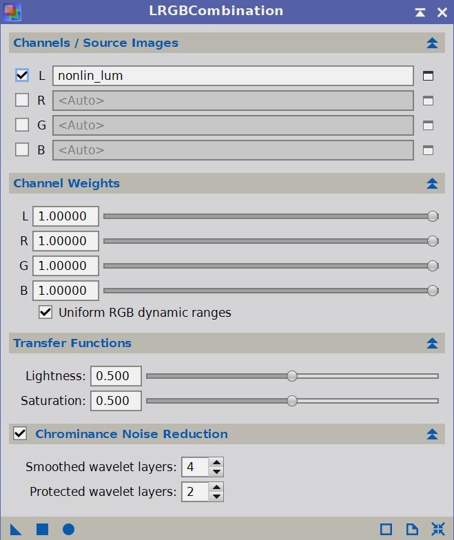
The LRGBCombination tool was used to fold the Lum image into the HaRGB image.
HaRGB nonlin image before Lum integration (click to enlarge)
After the Lum image was injected. (click to enlarge)
15. Process the LHaRGB image further

Apply CT to tweak tone scale and color sat
Use Color Sat to reduce green, boost red and blue
Create a red mask with the ColorMask script
red color
blur levels: 2
Run deconvolution with stddev = 10, apply twice
Tweak contrast and sat slightly with CT
Apply SCNR to remove any green casts
Rotate the image 180 degrees for a better composition
Create a mask covering the galaxy body with the GAME script
Apply and just tone scale and sat with CT
Run HRDMT with eight layers to compress the core region
Run CT to restore some lost contrast lost with HDRMT
Apply LHE with a radius of 326, a contrast limit of 2.0, an amount of 0.4, using a 12-bit histogram
15. Apply Nonlinear Noise Reduction
Setup ACDNR Lightness Panel as shown
Setup ACDNR Chrominance panel as shown
Select several previews and test
Apply to image

FInal setup for ACDNR Lightness

Final setup for ACDNR Chrominance
LHaRGB image before ACDNR application
After ACDNR Application.
16. Enhance Dark Structure
Apply DarkStructuresEnhance script with defaults.
17. Star Reduction
Use EZ-StarReduction script with Adam Block method to reduce stars
Before EZ-StarReduction (click to enlarge)
After EZ-StarReduction (click to enlarge)
18. Move to PhotoShop
Export as 16-bit tiff
Open in Photoshop
Use Camera Raw filter to tweak color, tone, and CLarity
Use Starshrink to reduce small stars
Use Starshrink to reduce large stars
Select the Red side blue side of the galaxy with a 100-pixel feather, add a slight red curve
Select the outer clouds and boost blue
Add watermarks
Export various versions of the image
More Info
Wikipedia: Messier 31
NASA: Take a "Swift" Tour of the Andromeda Galaxy
Carnegie Science: Hubble's Famous M31 VAR! plate
The SkyLive: Messier 31
Capture Details
Lights
Number of frames is after bad or questionable frames were culled.
48 x 90 seconds, bin 1x1 @ -15C, unity gain, ZWO Gen II L Filter
47 x 90 seconds, bin 1x1 @ -15C, 0 gain, ZWO Gen II R Filter
40 x 90 seconds, bin 1x1 @ -15C, unity gain, ZWO Gen II G Filter
37 x 90 seconds, bin 1x1 @ -15C, unity gain, ZWO Gen II B Filter
21 x 300 seconds, bin 1x1 @ -15C, unity gain, Astronomiks 6nm Ha Filter
Total of 6 hours 3 minutes
Cal Frames
25 Darks at 300 seconds, bin 1x1, -15C, gain 0
50 Darks at 90 seconds, bin 1x1, -15C, gain 0
25 Dark Flats at each Flat exposure times, bin 1x1, -15C, gain 0
15 R Flats
15 G Flats
15 B Flats
15 L Flats
15 Ha Flats
Capture Hardware:
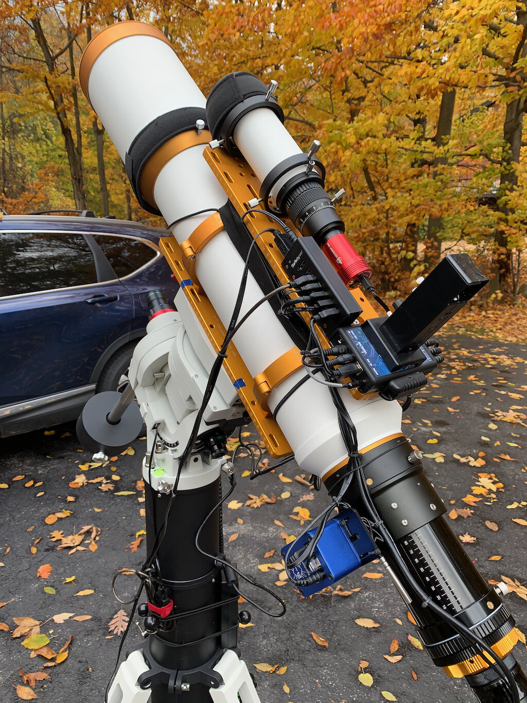
Scope: Askar FRA400 73MM F/5 Quintuplet Astrograph
Guide Scope: William Optics 50mm
Camera: ZWO ASI1600mm-pro with ZWO Filter wheel with ZWO LRGB filter set, and Astronomiks 6nm Narrowband filter set
Guide Camera: ZWO ASI290Mini
Focus Motor: Pegasus ZWO EAF 5V
Mount: Ioptron CEM 26
Polar Alignment: Ipolar camera
Software:
Capture Software: PHD2 Guider, Sequence Generator Pro controller
Image Processing: Pixinsight, Photoshop - assisted by Coffee, extensive processing indecision and second-guessing, editor regret and much swearing…..
The portable scope platform is supposed to be, well, portable. That means light and compact. In determining how to pack this platform for travel, I realized that the finder scope mounting rings made no sense in this application and I changed them out with something both more rigid and compact - the William Optics 50mm base-slide ring set.