Methods for Speech Quantization and Error Correction
This invention relates to methods for quantizing speech and for preserving the quality of speech during the presence of bit errors.
Relevant publications include: J. L. Flanagan, Speech Analysis, Synthesis and Perception, Springer- Verlag, 1972, pp. 378-386, (discusses phase vocoder - frequencybased speech analysis-synthesis system); Quatieri, et al., "Speech Transformations Based on a Sinusoidal Representation", IEEE TASSP, Vol, ASSP34, No. 6, Dec. 1986, pp. 1449-1986, (discusses analysis-synthesis technique based on a sinusoidal representation); Griffi n, "Multiband Excitation Vocoder", Ph.D. Thesis, M.I.T, 1987, (discusses an 8000 bps Multi-Band Excitation speech coder); Griffi n, et al, "A High Quality 9.6 kbps Speech Coding System", Proc. ICASSP 86, pp. 125-128, Tokyo, Japan, April 13-20, 1986, (discusses a 9600 bps Multi-Band Excitation speech coder); Griffi n, et al., "A New Model-Based Speech Analysis/Synthesis System", Proc. ICASSP 85. pp. 513-516. Tampa. FL., March 26-29. 19S5, (discusses Multi-Band Excitation speech model); Hardwick, "A 4.8 kbps Multi-Band Excitation Speech Coder", S.M. Thesis, M.I.T, May 1988, (discusses a 4800 bps Multi-Band Excitation speech coder); McAulay et al., "Mid- Rate Coding Based on a Sinusoidal Representation of Speech", Proc. ICASSP 85, pp. 945-948, Tampa, FL., March 26-29, 1985, (discusses speech coding based on a sinusoidal representation); Campbell et al., "The New 4800 bps Voice Coding Standard", Mil Speech Tech Conference, Nov. 1989, (discusses error correction in low rate speech coders); Campbell et al., "CELP Coding for Land Mobile Radio Applications", Proc. ICASSP 90, pp. 465-468, Albequerque, NM. April 3-6, 1990, (discusses error correction in low rate speech coders); Levesque et al., Error-Control Techniques for Digital Communication, Wiley, 1985, pp. 157-170, (discusses error correction in general); Jayant et al., Digital Coding of Waveforms, Prentice-Hall, 1984 (discusses quantization in general); Makhoul, et.al. "Vector Quantization in Speech Coding", Proc. IEEE, 1985, pp. 1551-1588 (discusses vector
quantization in general); Jayant et al., "Adaptive Postfiltering of 16 kb/s-ADPCM Speech", Proc. ICASSP 86, pp. 829-832, Tokyo, Japan, April 13-20, 1986, (discusses adaptive postfiltering of speech). The contents of these publications axe incorporated herein by reference.
The problem of speech coding (compressing speech into a small number of bits) has a large number of applications, and as a result has received considerable attention in the literature. One class of speech coders (vocoders) which have been extensively studied and used in practice is based on an underlying model of speech. Examples from this class of vocoders include linear prediction vocoders, homomorphic vocoders, and channel vocoders. In these vocoders, speech is modeled on a short-time basis as the response of a linear system excited by a periodic impulse train for voiced sounds or random noise for unvoiced sounds. For this class of vocoders, speech is analyzed by first segmenting speech using a window such as a Hamming window. Then, for each segment of speech, the excitation parameters and system parameters are estimated and quantized. The excitation parameters consist of the voiced/unvoiced decision ahd the pitch period. The system parameters consist of the spectral envelope or the impulse response of the system. In order to reconstruct speech, the quantized excitation parameters are used to synthesize an excitation signal consisting of a periodic impulse train in voiced regions or random noise in unvoiced regions. This excitation signal is then filtered using the quantized system parameters.
Even though vocoders based on this underlying speech model have been quite successful in producing intelligible speech, they have not been successful in producing high-quality speech. As a consequence, they have not been widely used for high- quality speech coding. The poor quality of the reconstructed speech is in part due to the inaccurate estimation of the model parameters and in part due to limitations in the speech model.
A new speech model, referred to as the Multi-Band Excitation (MBE) speech
model, was developed by Griffi n and Lim in 1984. Speech coders based on this new speech model were developed by Griffin and Lim in 1986, and they were shown to be capable of producing high quality speech at rates above 8000 bps (bits per second). Subsequent work by Hardwick and Lim produced a 4800 bps MBE speech coder which was also capable of producing high quality speech. This 4800 bps speech coder used more sophisticated quantization techniques to achieve similar quality at 4800 bps that earlier MBE speech coders had achieved at 8000 bps.
The 4800 bps MBE speech coder used a MBE analysis/synthesis system to estimate the MBE speech model parameters and to synthesize speech from the estimated MBE speech model parameters. A discrete speech signal, denoted by s(n), is obtained by sampling an analog speech signal. This is typically done at an 8 kHz. sampling rate, although other sampling rates can easily be accommodated through a straightforward change in the various system parameters. The system divides the discrete speech signal into small overlapping segments or segments by multiplying s(n) with a window w(n) (such as a Hamming window or a Kaiser window) to obtain a windowed signal sw(n). Each speech segment is then analyzed to obtain a set of MBE speech model parameters which characterize that segment. The MBE speech model parameters consist of a fundamental frequency, which is equivalent to the pitch period, a set of voiced/unvoiced decisions, a set of spectral amplitudes, and optionally a set of spectral phases. These model parameters are then quantized using a fixed number of bits for each segment. The resulting bits can then be used to reconstruct the speech signal, by first reconstructing the MBE model parameters from the bits and then synthesizing the speech from the model parameters. A block diagram of a typical MBE speech coder is shown in Figure 1.
The 4800 bps MBE speech coder required the use of a sophisticated technique to quantize the spectral amplitudes. For each speech segment the number of bits which could be used to quantize the spectral amplitudes varied between 50 and 125 bits. In
addition the number of spectral amplitudes for each segment varies between 9 and 60. A quantization method was devised which could efficiently represent all of the spectral amplitudes with the number of bits available for each segment. Although this spectral amplitude quantization method was designed for use in an MBE speech coder the quantization techniques axe equally useful in a number of different speech coding methods, such as the Sinusoidal Transform Coder and the Harmonic Coder . For a particular speech segment
denotes the number of spectral amplitudes in that segment. The value of
is derived from the fundamental frequency,
, according to the relationship,
where 0≤ β≤ 1.0 determines the speech bandwidth relative to half the sampling rate. The function [x], referred to in Equation (1), is equal to the largest integer less than or equal to x. The
spectral amplitudes are denoted by for 1≤ /≤
where is the lowest frequency spectral amplitude and is the highest frequency
spectral amplitude.
The spectral amplitudes for the current speech segment are quantized by first calculating a set of prediction residuals which indicate the amount the spectral amplitudes have changed between the current speech segment and the previous speech segment. If
denotes the number of spectral amplitudes in the current speech segment and
denotes the number of spectral amplitudes in the previous speech segment, then the prediction residuals,
for 1≤ /≤
axe given by,
where denotes the spectral amplitudes of the current speech segment and
denotes the quantized spectral amplitudes of the previous speech segment. The constant 7 is typically equal to .7, however any value in the range 0≤ 7≤ 1 can be used.
The prediction residuals are divided into blocks of K elements, where the value of K is typically in the range 4≤ K≤ 12. If is not evenly divisible by K, then the highest frequency block will contain less than K elements. This is shown in Figure 2 for = 34 and K = 8.
Each of the prediction residual blocks is then transformed using a Discrete Cosine
Transform (DCT) defined by,
The length of the transform for each block, J, is equal to the number of elements in the block. Therefore, all but the highest frequency block are transformed with a DCT of length A , while the length of the DCT for the highest frequency block is less than or equal to K. Since the DCT is an invertible transform, the
DCT coeffi cients completely specify the spectral amplitude prediction residuals for the current segment.
The total number of bits available for quantizing the spectral amplitudes is divided among the DCT coeffi cients according to a bit allocation rule. This rule attempts to give more bits to the perceptually more important low-frequency blocks, than to the perceptually less important high-frequency blocks. In addition the bit allocation rule divides the bits within a block to the DCT coeffi cients according to their relative long-term variances. This approach matches the bit allocation with the perceptual characteristics of speech and with the quantization properties of the DCT.
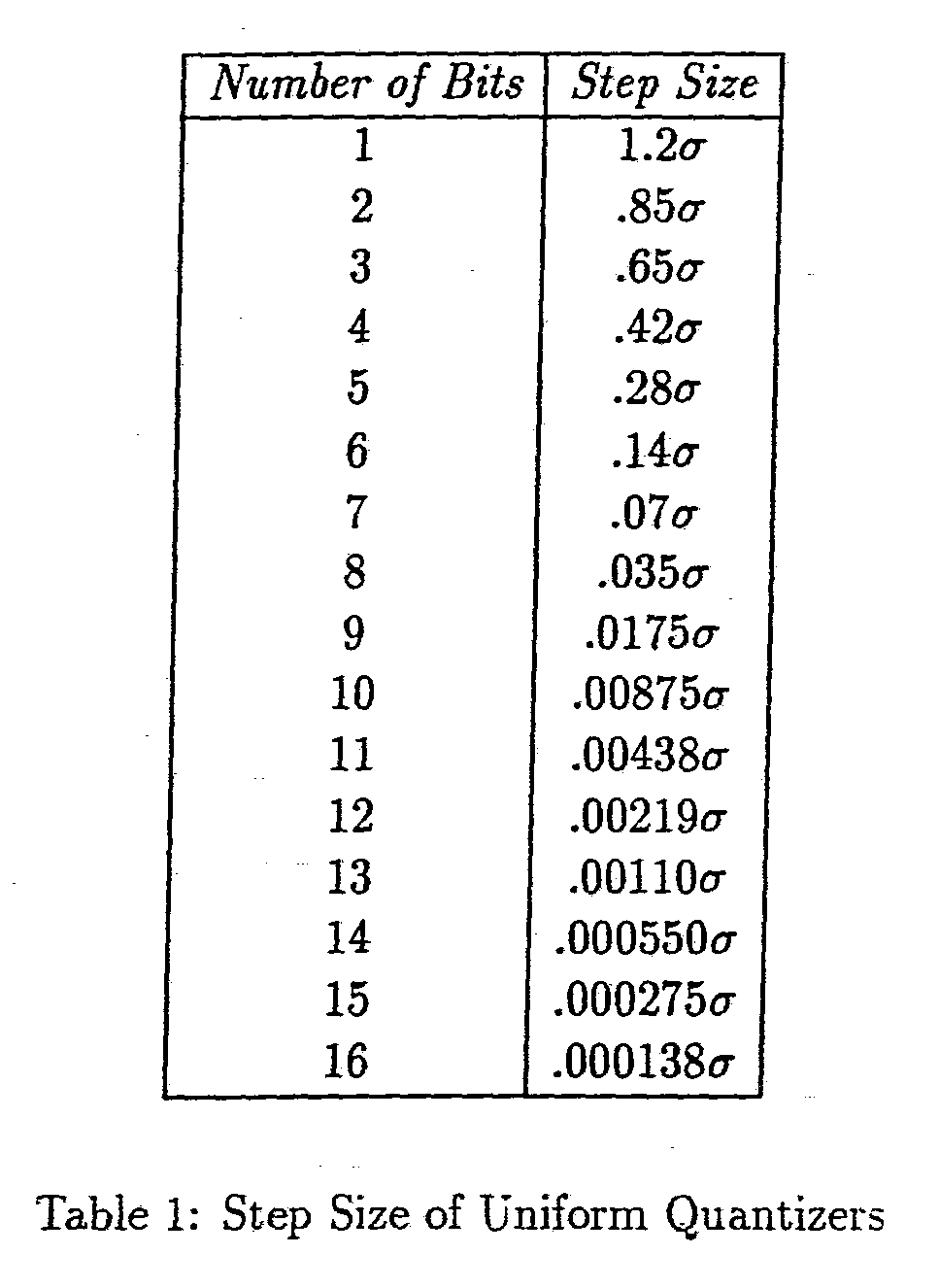
Each DCT coeffi cient is quantized using the number of bits specified by the bit allocation rule. Typically, uniform quantization is used, however non-uniform or vector quantization can also be used. The step size for each quantizer is determined from the long-term variance of the DCT coeffi cients and from the number of bits used to quantize each coeffi cient. Table 1 shows the typical variation in the step size as a function of the number of bits, for a long-term variance equal to σ2.
Once each DCT coeffi cient has been quantized using the number of bits specified by the bit allocation rule, the binary representation can be transmitted, stored, etc.,
depending on the application. The spectral amplitudes can be reconstructed from the binary representation by first reconstructing the quantized DCT coefficients for each block, performing the inverse DCT on each block, and then combining with the quantized spectral amplitudes of the previous segment using the inverse of Equation (2). The inverse DCT is given by,
where the length, J, for each block is chosen to be the number of elements in that block, a(j) is given by,
One potential problem with the 4800 bps MBE speech coder is that the perceived quality of the reconstructed speech may be significantly reduced if bit errors are added
to the binary representation of the MBE model parameters. Since bit errors exist in many speech coder applications, a robust speech coder must be able to correct, detect and/or tolerate bit errors. One technique which has been found to be very successful is to use error correction codes in the binary representation of the model parameters. Error correction codes allow infrequent bit errors to be corrected, and they allow the system to estimate the error rate. The estimate of the error rate can then be used to adaptively process the model parameters to reduce the effect of any remaining bit errors. Typically, the error rate is estimated by counting the number of errors corrected (or detected) by the error correction codes in the current segment, and then using this information to update the current estimate of error rate. For example if each segment contains a (23,12) Golay code which can correct three errors out of the 23 bits, and ej denotes the number of errors (0-3) which were corrected in the current segment, then the current estimate of the error rate, e
/-*, is updated according to:
where β is a constant in the range 0≤ β≤ 1 which controls the adaptability of∊R.
When error correction codes or error detection codes are used, the bits representing the speech model parameters are converted to another set of bits which are more robust to bit errors. The use of error correction or detection codes typically increases the number of bits which must be transmitted or stored. The number of extra bits which must be transmitted is usually related to the robustness of the error correction or detection code. In most applications, it is desirable to minimize the total number of bits which are transmitted or stored. In this case the error correction or detection codes must be selected to maximize the overall system performance.
Another problem in this class of speech coding systems is that limitations in the estimation of the speech model parameters may cause quality degradation in the synthesized speech. Subsequent quantization of the model parameters induces further degradation. This degradation can take the form of reverberant or muffled
quality to the synthesized speech. In addition background noise or other artifacts may be present which did not exist in the orignal speech. This form of degradation occurs even if no bit errors are present in the speech data, however bit errors can make this problem worse. Typically speech coding systems attempt to optimize the parameter estimators and parameter quantizers to minimize this form of degradation. Other systems attempt to reduce the degradations by post-filtering. In post-filtering the output speech is filtered in the time domain with an adaptive all-pole filter to sharpen the format peaks. This method does not allow fine control over the spectral enhancement process and it is computationally expensive and inefficient for frequency domain speech coders.
The invention described herein applies to many different speech coding methods, which include but are not limited to linear predictive speech coders, channel vocoders, homomorphic vocoders, sinusoidal transform coders, multi-band excitation speech coders and improved multiband excitation (IMBE) speech coders. For the purpose of describing this invention in detail, we use the 6.4 kbps IMBE speech coder which has recently been standardized as part of the INMARSAT-M (International Marine Satellite Organization) satellite communication system. This coder uses a robust speech model which is referred to as the Multi-Band Excitation (MBE) speech model.
Efficient methods for quantizing the MBE model parameters have been developed. These methods are capable of quantizing the model parameters at virtually any bit rate above 2 kbps. The 6.4 kbps IMBE speech coder used in the INMARSAT-M satellite communication system uses a 50 Hz frame rate. Therefore 128 bits are available per frame. Of these 128 bits, 45 bits are reserved for forward error correction. The remaining 83 bits per frame are used to quantize the MBE model parameters, which consist of a fundamental frequency ŵ
o, a set of V/UV decisions û
k for
≤ ≤ , and a set of spectral amplitudes
f or
The values of
K and
vary depending on the fundamental frequency of each frame. The 83 available bits are
divided among the model parameters as shown in Table 2.
The fundamental frequency is quantized by first converting it to its equivalent pitch period using Equation (7).
The value of
is typically restricted to the range
assuming an 8 kHz sampling rate. In the 6.4 kbps IMBE system this parameter is uniformly quantized using 8 bits and a step size of .5. This corresponds to a pitch accuracy of one half sample.
The V/UV decisions are binary values. Therefore they can be encoded using a single bit per decision. The 6.4 kbps system uses a maximum of 12 decisions, and the width of each frequency band is equal to 3ŵo. The width of the highest frequency band is adjusted to include frequencies up to 3.8 kHz.
The spectral amplitudes are quantized by forming a set of prediction residuals. Each prediction residual is the difference between the logarithm of the spectral amplitude for the current frame and the logarithm of the spectral amplitude representing the same frequency in the previous speech frame. The spectral amplitude prediction residuals are then divided into six blocks each containing approximately the same number of prediction residuals. Each of the six blocks is then transformed with a Discrete Cosine Transform (DCT) and the D.C. coefficients from each of the six blocks are combined into a 6 element Prediction Residual Block Average (PRBA)
vector. The mean is subtracted from the PRBA vector and quantized using a 6 bit non-uniform quantizer. The zero-mean PRBA vector is then vector quantized using a 10 bit vector quantizer. The 10 bit PRBA codebook was designed using a k-means clustering algorithm on a large training set consisting of zero-mean PRBA vectors from a variety of speech material. The higher-order DCT coefficients which are not included in the PRBA vector are quantized with scalar uniform quantizers using the 59 - remaining bits. The bit allocation and quantizer step sizes are based upon the long-term variances of the higher order DCT coefficients.
There are several advantages to this quantization method. First, it provides very good fidelity using a small number of bits and it maintains this fidelity as L varies over its range. In addition the computational requirements of this approach are well within the limits required for real-time implementation using a single DSP such as the AT&T DSP32C. Finally this quantization method separates the spectral amplitudes into a few components, such as the mean of the PRBA vector, which are sensitive to bit errors, and a large number of other components which are not very sensitive to bit errors. Forward error correction can then be used in an efficient manner by providing a high degree of protection for the few sensitive components and a lesser degree of protection for the remaining components. This is discussed in the next section.
In a first aspect, the invention features an improved method for forming the pre- dieted spectral amplitudes. They axe based on interpolating the spectral amplitudes of a previous segment to estimate the spectral amplitudes in the previous segment at the frequencies of the current segment. This new method corrects for shifts in the frequencies of the spectral amplitudes between segments, with the result that the prediction residuals have a lower variance, and therefore can be quantized with less distortion for a given number of bits. In preferred embodiments, the frequencies of the spectral amplitudes axe the fundamental frequency and multiples thereof.
In a second aspect, the invention features an improved method for dividing the
prediction residuals into blocks. Instead of fixing the length of each block and then dividing the prediction residuals into a variable number of blocks, the prediction residuals are divided into a predetermined number of blocks and the size of the blocks varies from segment to segment. In preferred embodiments, six (6) blocks are used in all segments; the number of prediction residuals in a lower frequency block is not larger that the number of prediction residuals in a higher frequency block; the difference between the number of elements in the highest frqeuency block and the number of elements in the lowest frequency block is less than or equal to one. This new method more closely matches the characteristics of speech, and therefore it allows the prediction residuals to be quantized with less distortion for a given number of bits. In addition it can easily be used with vector quantization to further improve the quantization of the spectral amplitudes.
In a third aspect, the invention features an improved method for quantizing the prediction residuals. The prediction residuals are grouped into blocks, the average of the prediction residuals within each block is determined, the averages of all of the blocks are grouped into a prediction residual block average (PRBA) vector, and the
PRBA vector is encoded. In preferred embodiments, the average of the prediction residuals is obtained by adding the spectral amplitude prediction residuals within the block and dividing by the number of prediction residuals within that block, or by computing the DCT of the spectral amplitude prediction residuals within a block and using the first coeffi cient of the DCT as the average. The PRBA vector is preferably encoded using one of two methods: (1) performing a transform such as the DCT on the PRBA vector and scalar quantizing the transform coeffi cients; (2) vector quantizing the PRBA vector. Vector quantization is preferably performed by determining the average of the PRBA vector, quantizing said average using scalar quantization, and quantizing the zero-mean PRBA vector using vector quantization with a zero-mean code-book. An advantage of this aspect of the invention is that it
allows the prediction residuals to be quantized with less distortion for a given number of bits.
In a fourth aspect, the invention features an improved method for determining the voiced/unvoiced decisions in the presence of a high bit error rate. The bit error rate is estimated for a current speech segment and compared to a predetermined error-rate threshold, and the voiced/unvoiced decisions for spectral amplitudes above a predetermined energy threshold are all declared voiced for the current segment when the estimated bit error rate is above the error-rate threshold. This reduces the perceptual effect of bit errors. Distortions caused by switching from voiced to unvoiced are reduced.
In a fifth aspect, the invention features an improved method for error correction (or error detection) coding of the speech model parameters. The new method uses at least two types of error correction coding to code the quantized model parameters. A first type of coding, which adds a greater number of additional bits than a second type of coding, is used for a group of parameters that is more sensitive to bit errors. The other type of error correction coding is used for a second group of parameters that is less sensitive to bit errors than the first. Compared to existing methods, the new method improves the quality of the synthesized speech in the presence of bit errors while reducing the amount of additional error correction or detection bits which must be added. In preferred embodiments, the different types of error correction include Golay codes and Hamming codes.
In a sixth aspect, the invention features a further method for improving the quality of synthesized speech in the presence of bit errors. The error rate is estimated from the error correction coding, and one or more model parameters from a previous segment are repeated in a current segment when the error rate for the parameters exceeds a predetermined level. In preferred embodiments, all of the model parameters are repeated.
In a seventh aspect, the invention features a new method for reducing the degradation caused by the estimation and quantization of the model parameters. This new method uses a frequency domain representation of the spectral envelope parameters to enhance regions of the spectrum which are perceptually important and to attenuate regions of the spectrum which axe perceptually insignificant. The result is that degradaion in the synthesized speech is reduced. A smoothed spectral envelope of the segment is generated by smoothing the spectral envelope, and an enhanced spectral envelope is generated by increasing some frequency regions of the spectral envelope for which the spectral envelope has greater amplitude than the smoothed envelope and decreasing some frequency regions for which the spectral envelope has lesser amplitude than the smoothed envelope. In preferred embodiments, the smoothed spectral envelope is generated by estimating a low-order model (e.g. an all-pole model) from the spectral envelope. Compared to existing methods this new method is more computationally effi cient for frequency domain speech coders. In addition this new method improves speech quality by removing the frequency domain constraints imposed by time-domain methods.
Other features and advantages of the invention will be apparent from the following description of preferred embodiments and from the claims.
Brief Description of the Drawings Figures 1-2 are diagrams showing prior art speech coding methods.
Figure 3 is a flow chart showing a preferred embodiment of the invention in which the spectral amplitude prediction accounts for any change in the fundamental frequency
Figure 4 is a flow chart showing a preferred embodiment of the invention in which the spectral amplitudes are divided into a fixed number of blocks
Figure 5 is a flow chart showing a preferred embodiment of the invention in which a prediction residual block average vector is formed.
Figure 6 is a flow chart showing a preferred embodiment of the invention in which the prediction residual block average vector is vector quantized
Figure 7 is a flow chart showing a preferred embodiment of the invention in which the prediction residual block average vector is quantized with a DCT and scalar quantization.
Figure 8 is a flow chart showing a preferred embodiment of the invention encoder in which different error correction codes are used for different model parameter bits.
Figure 9 is a flow chart showing a preferred embodiment of the invention decoder in which different error correction codes are used for different model parameter bits.
Figure 10 is a flow chart showing a preferred embodiment of the invention in which frequency domain spectral envelope parameter enhancement is depicted.
Description of Preferred Embodiments of the Invention
In the prior art, the spectral amplitude prediction residuals were formed using Equation (2). This method does not account for any change in the fundamental frequency between the previous segment and current segment. In order to account for the change in the fundamental frequency a new method has been developed which first interpolates the spectral amplitudes of the previous segment. This is typically done using linear interpolation, however various other forms of interpolation could also be used. Then the interpolated spectral amplitudes of the previous segment are resampled at the frequency points corresponding to the multiples of the fundamental frequency of the current segment. This combination of interpolation and resampling produces a set of predicted spectral amplitudes, which have been corrected for any inter-segment change in the fundamental frequency.
Typically a fraction of the base two logarithm of the predicted spectral amplitudes is subtracted from the base two logarithm of the spectral amplitudes of the current segment. If linear interpolation is used to compute the predicted spectral amplitudes,
then this can be expressed mathematically as:
where γ is a constant subject to 0 ≤ γ ≤ 1. Typically, γ = .7, however other values of γ can also be used. For example γ could be adaptively changed from segment to segment in order to improve performance. The parameters ŵo o and ŵo -1 in Equation (9) refer to the fundamental frequency of the current segment and the previous segment, respectively. In the case where the two fundamental frequencies are the same, the new method is identical to the old method. In other cases the new method produces a prediction residual with lower variance than the old method. This allows the prediction residuals to be quantized with less distortion for a given number of bits.
In another aspect of the invention a new method has been developed to divide the spectral amplitude prediction residuals into blocks. In the old method the
prediction residuals from the current segment were divided into blocks of K elements, where K = 8 is a typical value. Using this method, the characteristics of each block were found to be significantly different for large and small values of
. This reduced the quantization effi ciency, thereby increasing the distortion in the spectral amplitudes. In order to make the characteristics of each block more uniform, a new method was divised which divides the
prediction residuals into a fixed number of blocks. The length of each block is chosen such that all blocks within a segment have nearly the same length, and the sum of the lengths of all the blocks within a segment equal.
. Typically the total number of prediction residuals is divided into 6 blocks, where the length of each block is equal to
. If
is not evenly divisible by 6 then the length of one or more higher frequency blocks is increased by one, such that all of the spectral magnitudes are included in one of the six blocks. This new
method is shown in Figure 4 for the case where 6 blocks are used and L = 34. In this new method the approximate percentage of the prediction residuals contained in each block is independent of
This reduces the variation in the characteristics of each block, and it allows more effi cient quantization of the prediction residuals.
The quantization of the prediction residuals can be further improved by forming a prediction residual block average (PRBA) vector. The length of the PRBA vector is equal to the number of blocks in the current segment. The elements of this vector correspond to the average of the prediction residuals within each block. Since the first DCT coefficient is equal to the average (or D.C. value), the PRBA vector can be formed from the first DCT coefficient from each block. This is shown in Figure 5 for the case where 6 blocks axe present in the current segment and
This process can be generalized by forming additional vectors from the second (or third, fourth, etc.) DCT coefficient from each block.
The elements of the PRBA vector are highly correlated. Therefore a number of methods can be used to improve the quantization of the spectral amplitudes. One method which can be used to achieve very low distortion with a small number of bits is vector quantization. In this method a codebook is designed which contains a number of typical PRBA vectors. The PRBA vector for the current segment is compared against each of the codebook vectors, and the one with the lowest error is chosen as the quantized PRBA vector. The codebook index of the chosen vector is used to form the binary representation of the PRBA vector. A method for performing vector quantization of the PRBA vector has been developed which uses the cascade of a 6 bit non-uniform quantizer for the mean of the vector, and a 10 bit vector quantizer for the remaining information. This method is shown in Figure 6 for the case where the PRBA vector always contains 6 elements. Typical values for the 6 bit and 10 bit quantizers are given in the attached appendix.
An alternative method for quantizing the PRBA vector has also been developed.
This method requires less computation and storage than the vector quantization method. In this method the PRBA vector is first transformed with a DCT as defined in Equation (3). The length of the DCT is equal to the number of elements in the PRBA vector. The DCT coefficients are then quantized in a manner similar to that discussed in the prior art. First a bit allocation rule is used to distribute the total number of bits used to quantize the PRBA vector among the DCT coeffi cients. Scalar quantization (either uniform or non-uniform) is then used to quantize each DCT coeffi cient using the number of bits specified by the bit allocation rule. This is shown in Figure 7 for the case where the PRBA vector always contains 6 elements.
Various other methods can be used to effi ciently quantize the PRBA vector. For example other transforms such as the Discrete Fourier Transform, the Fast Fourier Transform, the Karhunen-Louve Transform could be used instead of the DCT. In addition vector quantization can be combined with the DCT or other transform. The improvements derived from this aspect of the invention can be used with a wide variety of quantization methods.
In another aspect a new method for reducing the perceptual effect of bit errors has been developed. Error correction codes are used as in the prior art to correct infrequent bit errors and to provide an estimate of the error rate∊
R. The new method uses the estimate of the error rate to smooth the voiced/unvoiced decisions, in order to reduce the perceived effect of any remaining bit errors. This is done by first comparing the error rate against a threshold which signifies the rate at which the distortion from uncorrected bit errors in the voiced/unvoiced decisions is significant. The exact value of this threshold depends on the amount of error correction applied to the voiced/unvoiced decisions, but a threshold value of .003 is typical if little error correction has been applied. If the estimated error rate,∊
R, is below this threshold then the voiced/unvoiced decisions are not perturbed. If ∊
R is above this threshold
then every spectral amplitude for which Equation (10) is satisfied is declared voiced.
Although Equation (10) assumes a threshold value of .003, this method can easily be modified to accommodate other thresholds. The parameter SE is a measure of the local average energy contained in the spectral amplitudes. This parameter is typically updated each segment according to:
The initial value of SE is set to an arbitrary initial value in the range 0≤ SE≤ 10000.0. The purpose of this parameter is to reduce the dependency of Equation (10) on the average signal level. This ensures that the new method works as well for low- level signals as it does for high level signals.
The specific forms of Equations (10), (11) and (12) and the constants contained within them can easily be modified, while maintaining the essential components of the new method. The main components of this new method are to first use an estimate of the error rate to determine whether the voiced/unvoiced decisions need to be smoothed. Then if smoothing is required, the voiced/unvoiced decisions are perturbed such that all high energy spectral amplitudes are declared voiced. This eliminates any high energy voiced to unvoiced or unvoiced to voiced transitions between segments, and as a result it improves the perceived quality of the reconstructed speech in the presence of bit errors.
In our invention we divide the quantized speech model parameter bits into three or more different groups according to their sensitivity to bit errors, and then we
use different error correction or detection codes for each group. Typically the group of data bits which is determined to be most sensitive to bit errors is protected using very effective error correction codes. Less effective error correction or detection codes, which require fewer additional bits, are used to protect the less sensitive data bits. This new method allows the amount of error correction or detection given to each group to be matched to its sensitivity to bit errors. Compared to the prior art, this method has the advantage that the degradation caused by bit errors is reduced and the number of bits required for forward error correction is also reduced.
The particular choice of error correction or detection codes which is used depends upon the bit error statistics of the transmission or storage medium and the desired bit rate. The most sensitive group of bits is typically protected with an effective error correction code such as a Hamming code, a BCH code, a Golay code or a Reed- Solomon code. Less sensitive groups of data bits may use these codes or an error detection code. Finally the least sensitive groups may use error correction or detection codes or they may not use any form of error correction or detection. The invention is described herein using a particular choice of error correction and detection codes which was well suited to a 6.4 kbps IMBE speech coder for satellite communications.
In the 6.4 kbps IMBE speech coder, which was standardized for the INMARSATM satellite communciation system, the 45 bits per frame which are reserved for forward error correction are divided among [23,12] Golay codes which can correct up to 3 errors, [15,11] Hamming codes which can correct single errors and parity bits. The six most significant bits from the fundamental frequency and the three most significant bits from the mean of the PRBA vector are first combined with three parity check bits and then encoded in a [23,12] Golay code. A second Golay code is used to encode the three most significant bits from the PRBA vector and the nine most sensitive bits from the higher order DCT coeffi cients. All of the remaining bits except the seven least sensitive bits are then encoded into five [15,11] Hamming codes. The
seven least significant bits are not protected with error correction codes.
Prior to transmission the 128 bits which represent a particular speech segment are interleaved such that at least five bits separate any two bits from the same code word. This feature spreads the effect of short burst errors over several different codewords, thereby increasing the probability that the errors can be corrected.
At the decoder the received bits are passed through Golay and Hamming decoders which attempt to remove any bit errors from the data bits. The three parity check bits are checked and if no uncorrectable bit errors are detected then the received bits are used to reconstruct the MBE model parameters for the current frame. Otherwise if an uncorrectable bit error is detected then the received bits for the current frame are ignored and the model parameters from the previous frame are repeated for the current frame.
The use of frame repeats has been found to improve the perceptual quality of the speech when bit errors axe present. The invention examines each frame of received bits and determines whether the current frame is likely to contain a large number of uncorrectable bit errors. One method used to detect uncorrectable bit errors is to check extra parity bits which are inserted in the data. The invention also determines whether a large burst of bits errors has been encountered by comparing the number of correctable bit errors with the local estimate of the error rate. If the number of correctable bit errors is substantially greater than the local estimate of the error rate then a frame repeat is performed. Additionally, the invention checks each frame for invalid bit sequences (i.e. groups of bits which the encoder never transmits). If an invalid bit sequence is detected a frame repeat is performed.
The Golay and Hamming decoders also provide information on the number of correctable bit errors in the data. This information is used by the decoder to estimate the bit error rate. The estimate of the bit error rate is used to control adaptive smoothers which increase the perceived speech quality in the presence of uncorrectable
bit errors. In addition the estimate of the error rate can be used to perform frame repeats in bad error environments.
This aspect of the invention can be used with soft-decision coding to further improve performance. Soft-decision decoding uses additional information on the like- lihood of each bit being in error to improve the error correction and detection capabilities of many different codes. Since this additional information is often available from a demodulator in a digital communication system, it can provide improved robustness to bit errors without requiring additional bits for error protection.
The invention uses a new frequency domain parameter enhancement method which improves the quality of synthesized speech. The invention first locates the perceptually important regions of the speech spectrum. The invention then increases the amplitude of the perceptually important frequency regions relative to other frequency regions. The preferred method for performing frequency domain parameter enhancement is to smooth the spectral envelope to estimate the general shape of the spectrum. The spectrum can be smoothed by fitting a low-order model such as an all-pole model, a cepstral model, or a polynomial model to the spectral envelope. The smoothed spectral envelope is then compared against the unsmoothed spectral envelope and perceptually important spectral regions are identified as regions where the unsmoothed spectral envelope has greater energy than the smoothed spectral envelope. Similarly regions where the unsmoothed spectral envelope has less energy than the smoothed spectral envelope are identified as perceptually less important. Parameter enhancement is performed by increasing the amplitude of perceptually important frequency regions and decreasing the amplitude of perceptually less important frequency regions. This new enhancement method increases speech quality by eliminating or reducing many of the artifacts which are introduced during the estimation and quantization of the speech parameters. In addition this new method improves the speech intelligibility by sharpening the perceptually important speech formants.
In the IMBE speech decoder a first-order all-pole model is fit to the spectral envelope for each frame. This is done by estimating the correlation parameters, R
o and R
1 from the decoded model paxameters according to the following equations,
where M for
are the decoded spectral amplitudes for the current frame,
and ŵ
o is the decoded fundamental frequency for the current frame. The correlation parameters R
o and R
1 can be used to estimate a first-order all-pole model. This model is evaluated at the frequencies corresponding to the spectral amplitudes for the current frame
and used to generate a set of weights W
i according to the following formula.
These weights indicate the ratio of the smoothed all-pole spectrum to the IMBE spectral amplitudes. They are then used to individually control the amount of parameter enhancement which is applied to each spectral amplitude. This relationship is expressed in the following equation,
where for
are the enhanced spectral amplitudes for the current frame.
The enhanced spectral amplitudes are then used to perform speech synthesis. The use of the enhanced model parameters improves speech quahty relative to synthesis from the unenhanced model parameters.
Further description of the preferred embodiment is given in the attached Appendix.
INMARSAT M Voice Codec
©Copyright, Digital Voice Systems Inc., 1991
Version 1.7
13 September 1991
Digital Voice Systems Inc. (DVSI, U.S.A.) claims certain rights in the Improved Multi-Band Excitation voice coding algorithm described in this document and elsewhere in the INMARSAT M System Definition Manual. DVSI is willing to grant a royalty-free license to use the IMBE voice coding algorithm strictly in connection with the INMARSAT M system on certain conditions of reciprocity. Details may be obtained from INMARSAT.
This document may contain errors in the description of the IMBE voice coding algorithm. An attempt will be made to correct these errors in future updates of this document.
DVSI acknowledges the Massachusetts Institute of Technology where the Multi-Band Excitation speech model was developed. In addition DVSI acknowledges the Rome Air Development Center of the United States Air Force which supported the real-time hardware used "in the IN MARS AT/ AUS SAT voice coding evaluation.
Contents
1 Introduction 6 Multi-Band Excitation Speech Model 7 Speech Analysis 11
3.1 Pitch Estimation . . . . . . . . . . . . . . . . . . . . . . . . . . . . . . . . . 13
3.1.1 Determination of E(P) . . . . . . . . . . . . . . . . . . . . . . 15
3.1.2 Pitch Tracking . . . . . . . . . . . . . . . . . . . . . . . . . . . . . . 15
3.1.3 Look-Back Pitch Tracking . . . . . . . . . . . . . . . . . . . . . . . . 16
3.1.4 Look-Ahead Pitch Tracking . . . . . . . . . . . . . . . . . . . . . . . 17
3.1.5 Pitch Refinement . . . . . . . . . . . . . . . . . . . . . . . . . . . . . 19
3.2 Voiced/Unvoiced Determination . . . . . . . . . . . . . . . . . . . . . . . . . 21
3.3 Estimation of the Spectral Amplitudes . . . . . . . . . . . . . . . . . . . . . 23 Parameter Encoding and Decoding 25
4.1 Fundamental Frequency Encoding and Decoding . . . . . . . . . . . . . . . 25
4.2 Voiced/Unvoiced Decision Encoding and Decoding . . . . . . . . . . . . . . 27
4.3 Spectral Amplitudes Encoding . . . . . . . . . . . . . . . . . . . . . . . . . 27
4-3.1 Encoding the PRBA Vector . . . . . . . . . . . . . . . . . . . . . . . 31
4.3.2 Encoding the Higher Order DCT Coefficients . . . . . . . . . . . . . 32
4.4 Spectral Amplitudes Decoding . . . . . . . . . . . . . . . . . . . . . . . . 34
4.4.1 Decoding the PRBA Vector . . . . . . . . . . . . . . . . . . . . . . . 36
4.4.2 Decoding the Higher Order DCT Coefficients . . . . . . . . . . . . . 37
4.4.3 Spectral Amplitude Enhancement . . . . . . . . . . . . . . . . . . . 37 Forward Error Correction and Bit Interleaving 39
5.1 Error Correction Encoding . . . . . . . . . . . . . . . . . . . . . . . . . . . . 39
5.2 Bit Interleaving . . . . . . . . . . . . . . . . . . . . . . . . . . . . . . . . . . 42
5.3 Error Correction Decoding . . . . . . . . . . . . . . . . . . . . . . . . . . . . 42
5.4 Adaptive Smoothing . . . . . . . . . . . . . . . . . . . . . . . . . . . . . . . 43
6 Parameter Encoding Example 45
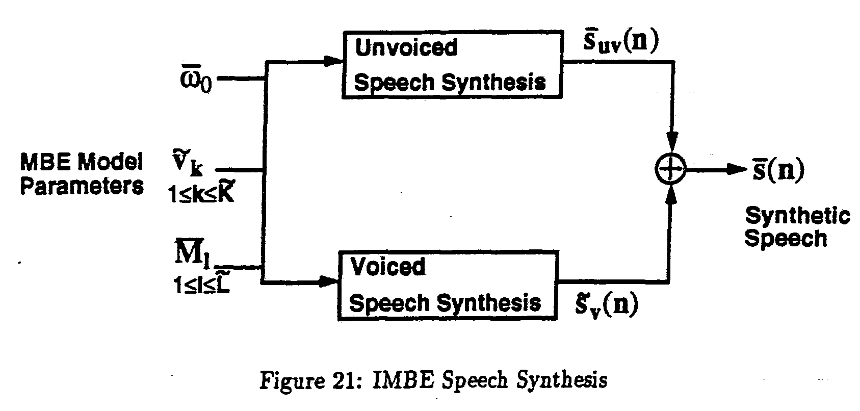
7 Speech Synthesis 51
7.1 Speech Synthesis Notation . . . . . . . . . . . . . . . . . . . . . . . . . . . . 51
7.2 Unvoiced Speech Synthesis . . . . . . . . . . . . . . . . . . . . . . . . . . . . 52
7.3 Voiced Speech Synthesis . . . . . . . . . . . . . . . . . . . . . . . . . . . . . 54
8 Additional Notes 57 A Variable Initialization 58 B Initial Pitch Estimation Window 59 C Pitch Refinement Window 61 D FIR Low Pass Filter 63 E Mean Prediction Residual Quantizer Levels 64 F Prediction Residual Block Average Quantization Vectors 65 G Spectral Amplitude Bit Allocation 97 H Bit Frame Format 118 I Speech Synthesis Window 120 J Flow Charts 122
List of Figures
1 Improved Multi-Band Excitation Speech Coder 7
2 Comparison of Traditional and MBE Speech Models 9
3 IMBE Speech Analysis Algorithm 11
4 High Pass Filter Frequency Response at 8 kHz. Sampling Rate 12
5 Relationship between Speech frames 13
6 Window Alignment 14
7 Initial Pitch Estimation 16
8 Pitch Refinement 19
9 IMBE Voiced/Unvoiced Determination 21
10 IMBE Frequency Band Structure 23
11 IMBE Spectral Amplitude Estimation 24
12 Fundamental Frequency Encoding and Decoding 27
13 V/UV Decision Encoding and Decoding 28
14 Encoding of the Spectral Amplitudes 28
15 Prediction Residual Blocks for L = 34 29
16 Formation of Prediction Residual Block Average Vector 30
17 Decoding of the Spectral Amplitudes 36
18 Error Correction Encoding 39
19 Format of û0 and ĉ0 41
20 Format of û1 and ĉ1 . 41
21 IMBE Speech Synthesis 52
List of Tables
1 Bit Allocation Among Model Parameters 25
2 Eight Bit Binary Representation 26
3 Standard Deviation of PRBA Quantization Errors 33
4 Step Size of Uniform Quantizers 33
5 Standard Deviation of DCT Coefficients for 1 < i < 6 34
Division of Prediction Residuals into Blocks in Encoding Example 45 Quantizers for
in Encoding Example 46 Quantizers for Ĉ
ij in Encoding Example 47 Construction of û
i in Encoding Example (1 of 3) 48 Construction of û
i in Encoding Example (2 of 3) 49 Constructioо of û
i in Encoding Example (3 of 3) 50 Breakdown of Algorithmic Delay 57
1 Introduction
This document provides a complete functional description of the INMARSAT-M speech coding algorithm. This document describes the essential operations which are necessary and sufficient to implement this algorithm. It is recommended that implementations begin with a high-level language simulation of the algorithm, and then proceed to a real-time implementation using a floating point digital signal processor such as the AT&T DSP32C, Motorola 96002 or TI TMS320C30 [2]. In addition it is highly recommended that the references be studied prior to the implementation of this algorithm.
The INMARSAT M speech coder is based upon the Improved Multi-Band Excitation (IMBE) speech coder [7]. This coder uses a new robust speech model which is referred to as the Multi-Band Excitation (MBE) speech model [5]. The basic methodology of the coder is to divide the speech signal into overlapping speech segments (or frames) using a window such as a Kaiser window. Each speech frame is then compared with the underlying speech model, and a set of model parameters are estimated for that particular frame. The encoder quantizes these model parameters and transmits a bit stream at 6.4 kbps. The decoder receives this bit stream, reconstructs the model parameters, and uses these model parameters to generate a synthetic speech signal. This synthesized speech signal is the output of the IMBE speech coder as shown in Figure 1.
The IMBE speech coder is a model-based speech coder, or vocoder. This means that the IMBE speech coder does not try to reproduce the input speech signal on a sample by sample basis. Instead the IMBE speech coder constructs a synthetic speech signal which contains the same perceptual information as the original speech signal. Many previous vocoders (such as LPC vocoders, homomorphic vocoders, and channel vocoders) have not been successful in producing high quality synthetic speech. The IMBE speech coder has two primary advantages over these vocoders. First, the IMBE speech coder is based on the MBE speech model which is a more robust model than the traditional speech models used in previous vocoders. Second, the IMBE speech coder uses more sophisticated algorithms to estimate the speech model parameters, and to synthesize the speech signal from these model parameters.
This document is organized as follows. In Section 2 the MBE speech model is briefly
discussed. Section 3 examines the methods used to estimate the speech model parameters, and Section 4 examines the quantization, encoding, decoding and reconstruction of the MBE model parameters. The error correction and the format of the 6.4 kbps bit stream is discussed in Section 5. This is followed by an example in Section 6, which demonstrates the encoding of a typical set of model parameters. Section 7 discusses the synthesis of speech from the MBE model parameters. A few additional comments on the algorithm and this document are provided in Section 8. The attached appendices provide necessary information such as the initialization for parameters. In addition Appendix J contains flow charts for some of the algorithms described in this document.
2 Multi-Band Excitation Speech Model
Let s(n) denote a discrete speech signal obtained by sampling an analog speech signal. In order to focus attention on a short segment of speech over which the model parameters are assumed to be constant, a window w(n) is applied to the speech signal s(n). The windowed
speech signal sw(n) is defined by sω( n) = s(n)ω(n) (1)
The sequence sw(n) is referred to as a speech segment or a speech frame. The IMBE analysis algorithm actually uses two different windows, ωR( n) and ωI(N), each of which is applied separately to the speech signal via Equation (1). This will be explained in more detail in Section 3 of this document. The speech signal s(n) is shifted in time to select any desired segment. For notational convenience sω(n) refers to the current speech frame. The next speech frame is obtained by shifting s(n) by 20 ms.
A speech segment sω(n) is modelled as the response of a hnear filter hω(n) to some excitation signal eω(n). Therefore, Sω(ω), the Fourier Transform of sω(n), can be expressed as
Sω(ω) = Hω{ω)Eω[ω) (2) where Hω(ω) and Ew(ω) are the Fourier Transforms of hω,(n) and ew(n), respectively.
In traditional speech models speech is divided into two classes depending upon the nature of the excitation signal. For voiced speech the excitation signal is a periodic impulse sequence, where the distance between impulses is the pitch period Po For unvoiced speech the excitation signal is a white noise sequence. The primary differences among traditional vocoders are in the method in which they model the linear filter hω(n). The spectrum of this filter is generally referred to as the spectral envelope of the speech signal. In a LPC vocoder, for example, the spectral envelope is modelled with a low order all-pole model. Similarly, in a homomorphic vocoder, the spectral envelope is modelled with a small number of cepstral coefficients.
The primary difference between traditional speech models and the MBE speech model is the excitation signal. In conventional speech models a single voiced/unvoiced (V/UV) decision is used for each speech segment. In contrast the MBE speech model divides the excitation spectrum into a number of non-overlapping frequency bands and makes a V/UV decision for each frequency band. This allows the excitation signal for a particular speech segment to be a mixture of periodic (voiced) energy and noise-like (unvoiced) energy. This added degree of freedom in the modelling of the excitation allows the MBE speech model
to generate higher quality speech than conventional speech models. In addition it allows the MBE speech model to be robust to the presence of background noise.
In the MBE speech model the exaltation spectrum is obtained from the pitch period (or the fundamental frequency) and the V/UV decisions. A periodic spectrum is used in the frequency bands declared voiced, while a random noise spectrum is used in the frequency bands declared unvoiced. The periodic spectrum is generated from a windowed periodic impulse train which is completely determined by the window and the pitch period. The random noise spectrum is generated from a windowed random noise sequence.
A comparison of a traditional speech model and the MBE speech model is shown in Figure 2. In this example the traditional model has classified the speech segment as voiced, and consequently the traditional speech model is comprised completely of periodic energy. The MBE model has divided the spectrum into 10 frequency bands in this example. The fourth, fifth, ninth and tenth bands have been declared unvoiced while the remaining bands have been declared voiced. The excitation in the MBE model is comprised of periodic energy only in the frequency bands declared voiced, while the remaining bands are comprised of
noise-like energy. This example shows an important feature of the MBE speech model. Namely, the V/UV determination is performed such that frequency bands where the ratio of periodic energy to noise-like energy is high are declared voiced, while frequency bands where this ratio is low are declared unvoiced. The details of this procedure are discussed in Section 3.2.
This section presents the methods used to estimate the MBE speech model parameters. To develop a high quality vocoder it is essential that robust and accurate algorithms are used to estimate the model parameters. The approach which is presented here differs from conventional approaches in a fundamental way. Typically algorithms for the estimation of the excitation parameters and algorithms for the estimation of the spectral envelope parameters operate independently. These parameters are usually estimated based on some reasonable but heuristic criterion without explicit consideration of how close the synthesized speech will be to the original speech. This can result in a synthetic spectrum quite different from the original spectrum. In the approach used in the IMBE speech coder the excitation and spectral envelope parameters are estimated simultaneously, so that the synthesized spectrum is closest in the least squares sense to the original speech spectrum. This approach can be viewed as an "analysis-by-synthesis" method. The theoretical derivation and justification of this approach is presented in references [5,6,8}.
A block diagram of the analysis algorithm is shown in Figure 3. The MBE speech model parameters which must be estimated for each speech frame are the pitch period (or equiva
lently the fundamental frequency), the V/UV decisions, and the spectral amplitudes which characterize the spectral envelope. A discrete speech signal is obtained by sampling an analog speech signal at 8 kHz. The speech signal should be scaled such that the maximum and minimum sample values are in the ranges [16383, 32767] and [-32768, -16385], respectively. In addition any non-linear companding which is introduced by the sampling system (such as a-law or u-law) should be removed prior to performing speech analysis.
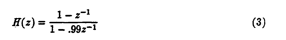
The discrete speech signal is first passed through a discrete high-pass filter with the following transfer function.
Figure 4 shows the frequency response of the filter specified in equation (3) assuming an 8 kHz. sampling rate. The resulting high-pass filtered signal is denoted by s(n) throughout the remainder of this section.
The organization of this section is as follows. Section 3.1 presents the pitch estimation algorithm. The V/UV determination is discussed in Section 3.2, and Section 3.3 discusses the estimation of the spectral amplitudes.
3.1 Pitch Estimation
The objective in pitch estimation is to determine the pitch P
o corresponding to the "current speech frame s
w(n). Po is related to the fundamental frequency ω
0 by
The pitch estimation algorithm attempts to preserve some continuity of the pitch between neighboring speech frames. A pitch tracking algorithm considers the pitch from previous and future frames, when determining the pitch of the current frame. The next speech frame is obtained by shifting the speech signal s(n) "left" by 160 samples (20 ms.) prior to the application of the window in Equation (1). The pitches corresponding to the next two speech frames are denoted by P1 and P2. Similarly, the previous frame is obtained by shifting -»(n) "right" by 160 samples prior to the application of the window. The pitches corresponding to the previous two speech frames axe denoted by P-1 and P-2. These relationships are shown in Figure 5.
The pitch is estimated using a two-step procedure. First an initial pitch estimate, denoted by
, is obtained. The initial pitch estimate is restricted to be a member of the set {21, 21.5, ... 113.5, 114}. It is then refined to obtain the final estimate of the fundamental frequency ŵ
o, which has one-quarter-sample accuracy. This two-part procedure is used in part to reduce the computational complexity, and in part to improve the robustness of the pitch estimate.
One important feature of the pitch estimation algorithm is that the initial pitch estima
tion algorithm uses a different window than the pitch refinement algorithm. The window used for Initial pitch estimation, ω/(n), is 281 samples long and is given in Appendix B. The window used for pitch refinement (and also for spectral amplitude estimation and V/UV determination), ωR(n), is 221 samples long and is given in Appendix C. Throughout this document the window functions are assumed to be equal to zero outside the range given in the Appendices. The center point of the two windows must coincide, therefore the first non-zero point of ωR(n) must begin 30 samples after the first non-zero point of ω/(n). This constraint is typically met by adopting the convention that ωR(n) = ωR(-n) and ωI(n) = ωI(n) , as shown in Figure 6. The amount of overlap between neighboring speech segments is a function of the window length. Specifically the overlap is equal to the window length minus the distance between frames (160 samples). Therefore the overlap when using ωR(n) is equal to 61 samples and the overlap when using ωI(n) is equal to 121 samples.
3.1.1 Determination of E(P)
To obtain the initial pitch estimate an error function, E(P), is evaluated for every P in the set {21, 21.5, ... 113.5, 114}. Pitch tracking is then used to compare the evaluations of E(P), and the best candidate from this set is chosen as
This procedure is shown in Figure 7. The function E(P) is defined by
M
where ω
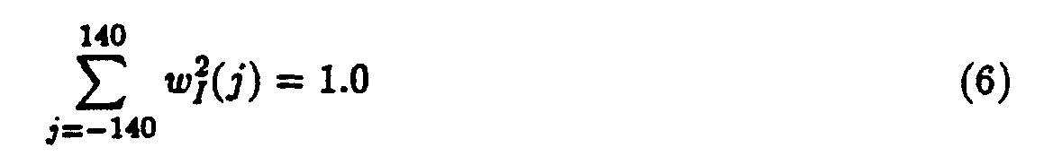
I(n) is normalized to meet the constraint
This constraint is satisfied for ωI(n) listed in Appendix B. The function r(t) is defined for integer values of t by 0
The function r(t) is evaluated at non-integer values of t through hnear interpolation:
where [x] is equal to the largest integer less than or equal to x (i.e. truncating values of x). The low-pass filtered speech signal is given by
where hLPF(n) is a 21 point FIR filter given in Appendix D.
The function E(P) in Equation (5) is derived in [5,8]. The initial pitch estimate
is chosen such that
is small, however, is not chosen simply to minimize E(P).
Instead pitch tracking must be used to account for pitch continuity between neighboring speech frames.
3.1.2 Pitch Tracking
Pitch tracking is used to improve the pitch estimate by attempting to limit the pitch deviation between consecutive frames. If the pitch estimate is chosen to strictly minimize E(P),
then the pitch estimate may change abruptly between succeeding frames. This abrupt change in the pitch can cause degradation in the synthesized speech. In addition, pitch typically changes slowly; therefore, the pitch estimates from neighboring frames can aid in estimating the pitch of the current frames.
For each speech frame two different pitch estimates are computed. The first, is a
backward estimate which maintains pitch continuity with previous speech frames. The second, , is a forward estimate which maintains pitch continuity with future speech frames. The backward pitch estimate is calculated with the look-back pitch tracking algorithm, while the forward pitch estimate is calculated with the look-ahead pitch tracking algorithm. These two estimates are compared with a set of decision rules defined below, and either the backward or forward estimate is chosen as the initial pitch estimate,
3.1.3 Look-Back Pitch Tracking
Let and P
denote the initial pitch estimates which are calculated during the analysis of the previous two speech frames. Let E
-1(P) and E
-2(P) denote the error functions of Equation (5) obtained from the analysis of these previous two frames as shown in Figure 5. Then
and
will have some specific values. Upon initialization the error functions E
-1(P) and E
-2(P) are assumed to be equal to zero, and
and
are assumed to be equal to 100.
Since pitch continuity with previous frames is desired, the pitch for the current speech frame is considered in a range near . First, the error function E(P) is evaluated at each
value of P which satisfies constraints (10) and (11).
P∈{21,21.5,...113.5, 114} (11)
These values of E(P) are compared and
is defined as the value of P which satisfies these constraints and which minimizes E(P). The backward cumulative error
is then computed using the following formula.
The backward cumulative error provides a confidence measure for the backward pitch estimate. It is compared against the forward cumulative error using a set of heuristics defined in Section 3.1.4. This comparison determines whether the forward pitch estimate or the backward pitch estimate is selected as the initial pitch estimate for the current frame.
3.1.4 Look-Ahead Pitch Tracking
Look-ahead tracking attempts to preserve pitch continuity between future speech frames. Let E1(P) and E2(P) denote the error functions of Equation (5) obtained from the two future speech frames as shown in Figure 5. Since the pitch has not been determined for these future frames, the look-ahead pitch tracking algorithm must select the pitch of these future frames. This is done in the Mowing manner. First, Po is assumed to be fixed. Then the P1 and P2 are found which jointly minimize E1(P1) + E2(P2), subject to constraints (13) through (16).
P1∊ {21,21.5,...113.5, 114} (13)
.8 · Po≤ P1≤1.2 · Po (14)
P2∈ {21,21.5,...113.5, 114} (15)
.8 ·P1≤P2≤ 1.2 · P1 (16)
The values of P
1 and P
1 which jointly minimize E
1(P
1)+ E
2(P
2) subject to these constraints are denoted by
and
respectively. Once
P and
have been computed the forward cumulative error function CEF(P
o) is computed according to:
This process is repeated for each P
0 in the set {21,21.5, ...113.5, 114}. The corresponding values of CE
F(P
0) axe compared and is defined as the value of P
0 in this set which results in the minimum value of CE
F(P
0).
Once has been found the integer sub-multiples of
must be considered. Every sub-multiple which is greater than or equal to 21 is computed and replaced with the closest member of the set {21, 21.5, ... 113.5, 114} (where closeness is measured with mean-square error). Sub-multiples which are less than 21 axe disregarded.
The smallest of these sub-multiples is checked against constraints (18), (19) and (20). If this sub-multiple satisfies any of these constraints then it is selected as the forward pitch estimate, Otherwise the next largest sub-multiple is checked against these constraints, and it is selected as the forward pitch estimate if it satisfies any of these constraints. This process continues until all pitch sub-multiples have been tested against these constraints. If no pitch sub-multiple satisfies any of these constraints then
Note that this procedure will always select the smallest sub-multiple which satisfies any of these constraints as the forward pitch estimate.
Once the forward pitch estimate and the backward pitch estimate have both been computed the forward cumulative error and the backward cumulative error are compared. Depending on the result of this comparison either
or
will be selected as the initial pitch estimate The following set of decision rules is used select the initial pitch estimate from among these two candidates.
This completes the initial pitch estimation algorithm. The initial pitch estimation,
is a member of the set {21, 21.5, ... 113.5, 114}, and therefore it has half-sample accuracy.
3.1.5 Pitch Refinement
The pitch refinement algorithm improves the resolution of the pitch estimate from one half sample to one quarter sample. Ten candidate pitches axe formed from the initial pitch estimate. These axe
These candidates are converted to their equivalent fundamental frequency using Equation (4). The error function E
R(ω
0), defined in Equation (24), is evaluated for each candidate fundamental frequency ωo. The candidate fundamental frequency which results in the minimum value of E
R(ω
0) is selected as the refined fundamental frequency
A block diagram of this process is shown in Figure 8 .
The synthetic spectrum -S
ω(m,ω
o) is given by,
where α
l, b
l and A
l axe defined in equations (26) thru (28), respectively. The notation [x] denotes the smallest integer greater than or equal to x.
The function Sω(m) refers to the 256 point Discrete Fourier Transform of s(n) · ωR(n), and WR(m) refers to the 16384 point Discrete Fourier Transform of ωR(n). These relationships are expressed below. Reference [15] should be consulted for more information on the DFT.
The notation WR*(m) refers to the complex conjugate of WR(m). However, since ωR(n) is a real symmetric sequence, WR*(m) = WR(m).
Once the refined fundamental frequency has been selected from among the ten candidates, it is used to compute the number of harmonics in the current segment, L, according to the relationship:
In addition the parameters
and
for
axe computed from ŵ
o according to equations (32) and (33), respectively.
3.2 Voiced/Unvoiced Determination
The voiced/unvoiced (V/UV) decisions,
for
axe found by dividing the spectrum into
frequency bands and evaluating a voicing measure, D
k, for each band. The number of frequency bands is a function of
and is given by:
The voicing measure for is given by
where ŵ
o is the refined fundamental frequency, and
, S
w(m), and S
w(m,ω
o) are defined in section 3.1.5. Similarly, the voicing measure for the highest frequency band is given by
The parameters Dk for
are compared with a threshold function
given by
The parameter ξ
o is equal to the energy of the current segment, and it is given by
The parameters ξαvg, ξmαx; and ξmin roughly correspond to the local average energy, the local maximum energy and the local minimum energy, respectively. These three paxameters are updated each speech frame according to the rules given below. The notation ξαvg(0), ξmαx(0) and ξmin(0) refers to the value of the parameters in the current frame, while the notation ξαvg(-1), ξmαx(-1) and ξmin(-1) refers to the value of the parameters in the previous frame.
After these parameters are updated, the two constraints expressed below are applied to ξmin(0) and ξmαx(0).
ξmin(0) = 200 if ξmin(0) < 200 (42) ξmαx(0) = 20000 if ξmαx(0) < 20000 (43)
The updated energy parameters for the current frame are used to calculate the function M(ξ0,ξαυg,ξmin,ξmαx). For notational convenience ξαυg, ξmin, and ξmαx refer to ξαvg(0), ξmin(0) and ξmαx(0), respectively.
The function M(ξ0,ξavg, ξmin,ξmαx) is used in Equation (37) to calculate the V/UV threshold function. If Dk is less than the threshold function then the frequency band
is declared voiced; otherwise this frequency band is declared unvoiced. A block diagram of this procedure is shown in Figure 9. The adopted convention is that if the frequency band
is declared voiced, then
Alternatively, if the frequency band
is declared unvoiced, then
With the exception of the highest frequency band, the width of each frequency band is equal to 3ŵ0. Therefore all but the highest frequency band contain three harmonics of the refined fundamental frequency. The highest frequency band (as defined by Equation (36))may contain more or less than three harmonics of the fundamental frequency. If a particular frequency band is declared voiced, then all of the harmonics within that band axe defined to be voiced harmonics. Similarly, if a particular frequency band is declared unvoiced, then all of the harmonics within that band are defined to be unvoiced harmonics.
3.3 Estimation of the Spectral Amplitudes
Once the V/UV decisions have been determined the spectral envelope can be estimated as shown in Figure 11. In the IMBE speech coder the spectral envelope in the frequency band fc is specified by 3 spectral amplitudes, which are denoted by
and The relationship between the frequency bands and the spectral amplitudes is shown in Figure 10. If the frequency band
is declared voiced, then
and are estimated by,
for I in the range 3ĸ - 2≤ /≤ 3ĸ and where A
ι(ω
o) is given in Equation (28). Alternatively, if the frequency band
is declared unvoiced, then
are estimated according to:
for / in the range 3ĸ - 2≤ /≤ 3ĸ.
This procedure must be modified slightly for the highest frequency band which covers the frequency interval
. The spectral envelope in this frequency band is represented by
spectral amplitudes, denoted If
this frequency band is declared voiced then these spectral amplitudes are estimated using equation (45) for
Alternatively, if this frequency band is declared unvoiced then these spectral amplitudes are estimated using equation (46) for
As described above, the spectral amplitude are estimated in the range
where is given in Equation (31). Note that the lowest frequency band, α
1≤ ω≤ b
3, is specified by
and
The D.C. spectral amplitude, M is ignored in the IMBE
speech coder and can be assumed to be zero.
4 Parameter Encoding and Decoding
The analysis of each speech frame generates a set of model parameters consisting of the fundamental frequency,
the V/UV decisions,
for
and the spectral amplitudes,
for
Since this voice codec is designed to operate at 6.4 kbps with a 20 ms. frame length, 128 bits per frame are available for encoding the model parameters. Of these 128 bits, 45 are reserved for error correction as is discussed in Section 5 of this document, and the remaining 83 bits are divided among the model parameters as shown in Table 1. This section describes the manner in which these bits are used to quantize, encode, decode and reconstruct the model parameters. In Section 4.1 the encoding and decoding of the fundamental frequency is discussed, while Section 4.2 discusses the encoding and decoding of the V/UV decisions. Section 4.3 discusses the quantization and encoding of the spectral amplitudes, and Section 4.4 discusses the decoding and reconstruction of the spectral amplitudes. Reference [9] provides general information on many of the techniques used in this section.
4.1 Fundamental Frequency Encoding and Decoding
The fundamental frequency is estimated with one-quarter sample resolution in the inter
however, it is only encoded at half-sample resolution. This is accomplished by finding the value of
which satisfies:
The quantity
can be represented with 8 bits using the unsigned binary representation shown in Table 2. This binary representation is used throughout the encoding and decoding
of the IMBE model parameters.
The fundamental frequency is decoded and reconstructed at the receiver by using Equation (48) to convert
to the received fundamental frequency
In addition
is used to calculate and
the number of V/UV decisions and the number of spectral amplitudes, respectively. These relationships are given in Equations (49) and (50).
Since and
control subsequent bit allocation by the receiver, it is important that they equal and
respectively. This occurs if there axe no uncorrectable bit errors in the six most significant bits (MSB) of
For this reason these six bits axe well protected by the error correction scheme discussed in Section 5. A block diagram of the fundamental frequency encoding and decoding process is shown in Figure 12.
Note that the encoder also uses equation (48) to reconstruct the fundamental frequency from as shown in Figure 12. This is necessary because the encoder needs
in order to compute the spectral amplitude prediction residuals via equations (53) through (54).
4.2 Voiced/Unvoiced Decision Encoding and Decoding
The V/UV decisions
for
axe binaxy values which classify each frequency band as either voiced or unvoiced. These values are encoded using
The encoded value
is represented with
bits using the binary representation shown in Table 2. At the receiver the
bits corresponding to
are decoded into the V/UV decisions for
This is done with the following equation.
If there axe no uncorrectable bit errors in
and if
then the transmitted V/UV decisions, will equal the received V/UV decisions
Figure 13 shows a block diagram of the V/UV decision encoding and decoding process.
4.3 Spectral Amplitudes Encoding
The spectral amplitudes
for
axe real values which must be quantized prior to encoding. This is accomplished as shown in Figure 14, by forming the prediction residuals for
according to Equations (53) through (54). For the purpose of this discussion
refers to the unquantized spectral amplitudes of the current frame,
refers to the quantized spectral amplitudes of the previous frame,
refers to the reconstructed fundamental frequency of the current frame and
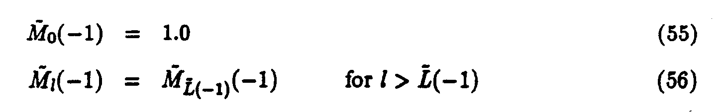
refers to the reconstructed fundamental frequency of the previous frame. Upon initialization
should be set equal to 1.0 for all I, and
.
In order to form
using equations (53) and (54), the following assumptions are always made:
The prediction residuals are then divided into 6 blocks. The length of each block, denoted for 1≤ i≤ 6, is adjusted such that the following constraints are satisfied.
The first or lowest frequency block is denoted by
for
and it consists of the first consecutive elements of
The second block is denoted by
for
and it consists of the next
consecutive elements of
This continues through the sixth or highest frequency block, which is denoted by
for
It consists of the last
consecutive elements of
An example of this process is shown in Figure 15 for
Each of the six blocks is transformed using a Discrete Cosine Transform (DCT), which is discussed in [9]. The length of the DCT for the i'th block is equal to The DCT
5
coefficients are denoted by
where 1≤ i≤ 6 refers to the block number, and
refers to the particular coefficient within each block. The formula for the computation of these DCT coefficients is as follows:
The DCT coefficients from each of the six blocks are then divided into two groups. The first group consists of the first DCT coefficient (i.e the D.C value) from each of the six blocks.
These coeffi cients are used to form a six element vector,
for 1≤ i≤ 6, where
The vector i is referred to as the Prediction Residual Block Average (PRBA) vector, and
its construction is shown in Figure 16. The quantization of the PRBA vector is discussed in section 4.3.1.
The second group consists of the remaining higher order DCT coefficients. These coefficients correspond to
where 1≤ t≤ 6 and
Note that if
then there axe no higher order DCT coefficients in the i'th block. The quantization of the higher order DCT coefficients is discussed in section 4.3.2.
One important feature of the spectral amplitude encoding algorithm, is that the spectral amplitude information is transmitted differentially. Specifically a prediction residual is
transmitted which measures the change in the spectral envelope between the current frame and the previous frame. In order for a differential scheme of this type to work properly, the encoder must simulate the operation of the decoder and use the reconstructed spectral amplitudes from the previous frame to predict the spectral amplitudes of the current frame. The IMBE spectral amplitude encoder simulates the spectral amplitude decoder by setting
and then reconstructing the spectral amplitudes as discussed above. This is shown as the feedback path in Figure 14.
4.3.1 Encoding the PRBA Vector
The PRBA vector is quantized using a three step procedure. First the vector mean πi
R is computed using equation (60), and it is scalar quantized using the 6 bit non- uniform quantizer defined in Appendix E. Next the PRBA vector is vector quantized using the 10 bit zero-mean codebook defined in Appendix F. Finally a six element quantization error vector,
for 1≤ *≤ 6 , is computed by adding the quantized vector mean to the selected entry from the 10 bit zero-mean codebook and then subtracting the result from the unquantized PRBA vector
. If then the six elements of axe scalar quantized
using uniform quantization. The step size and bit allocation for these uniform quantizers is documented later in this section. If
then
is disregarded.
The first step in quantizing the PRBA vector is to calculate the mean ITIR as defined in
The mean is scalar quantized by computing the mean square error between the unquantized mean and each of the 64 quantization levels listed in Appendix E. The 6 bit value
is defined as the index of the quantizer value (as shown in Appendix E) which is closest, in a mean-square error sense, to THR. It is represented using the same binary representation as is shown in Table 2.
After the mean is quantized the PRBA vector is vector quantized using the codebook listed in Appendix F. This is accomplished by computing the mean square error between the unquantized vector and each of the 1024 quantization vectors listed in Appendix F. Note that each of these quantization vectors has zero mean. The 10 bit value is defined
as the index of the quantization vector (as shown in Appendix F) which yields the minimum mean-square error, and it is represented using the same binary representation as is shown in Table 2. Additional information on vector quantization can be found in [12].
Finally the quantized mean from Appendix E is added to each element of the selected zero-mean quantization vector from Appendix F. The resulting vector is then subtracted from Ri to form the vector
Appendix G is then used to find the bit allocation for the six elements of this vector. This appendix lists the number of bits allocated to the values through which correspond to the elements through respectively. Note
that if then the bit allocation is equal to zero for these six elements. Each element
of is uniformly scalar quantized using a step size which is computed using Tables 3 and 4. Table 3 lists the standard deviation for the six elements of
while Table 4 lists the step size for each uniform quantizer as a function of the number of bits allocated to that
quantizer and the standard deviation of the element. For example if
is to be quantized using 3 bits, the step size is equal to .18 * .65 = .117. If the number of bits allocated to a particular element is greater than zero, then it is uniformly quantized using equation (61). Otherwise, if the number of bits allocated to a particular element is equal to zero, then that element is assumed to be equal to zero and is not encoded.
The parameters
and
in equation (61) refer to the bit encoding, the number of bits and the step size which has been computed for
respectively. Note that if the value of b is outside the range
then it is set equal to the closest value within this range. Finally, each encoding is converted into the appropriate binary representation using the same representation as is shown in Table 2.
4.3.2 Encoding the Higher Order DCT Coefficients
Once the PRBA vector has been quantized, the remaining bits are used to encode the
higher order DCT coefficients which complete the representation of the spectral amplitudes. Appendix G shows the bit allocation as a function of
for these coefficients. For each value of the first entries, labeled
through
provide the bit allocation for the higher
order DCT coefficients. The adopted convention is that correspond to
respectively.
Once the bit allocation for the higher order DCT coefficients has been obtained, these coefficients are quantized using uniform quantization. The step size used to quantize each coefficient is a function of the bit allocation and the standard deviation of the DCT coefficient. This relationship is summarized in Tables 4 and 5. For example, if 4 bits are allocated for a particular coefficient, then from Table 4 the step size,
equals .42σ. If this was the the third DCT coefficient from any block
then σ = .216 as shown in Table 5. This equates to a step size of .09072. If the number bits allocated to a particular coefficient is greater than zero, then that coefficient is encoded using equation (62). Otherwise, if the
number of bits allocated to a particular coefficient is equal to zero, then that element is assumed to be equal to zero and is not encoded.
The parameters
and
in equation (62) refer to the bit encoding, the number of bits and the step size which has been computed for
respectively. Note that if the value of is outside the range
then it is set equal to the closest value within this range. Finally, each encoding is converted into the appropriate binary representation using the same representation as is shown in Table 2.
4.4 Spectral Amplitudes Decoding
The spectral amplitudes are decoded and reconstructed by inverting the quantization and encoding procedure. First six blocks axe generated. The length of each block
for 1 < i≤ 6, is adjusted to meet the following constraints.
The elements of these blocks are denoted by
where 1 < i < 6 denotes the block number and where denotes the element within that block. The first element of each
block is then set equal to the decoded PRBA vector
via equation (65). The formation of the decoded PRBA vector is discussed in Section 4.4.1.
The remaining elements of each block correspond to the decoded higher order DCT coefficients which are discussed in Section 4.4.2.
Once the DCT coefficients
have been reconstructed, an inverse DCT is computed on each of the six blocks to form the vectors
This is done using the following equations for 1≤i≤ 6.
The six transformed blocks axe then joined to form a single vector of length which is
denoted for
The vector
corresponds to the reconstructed spectral amplitude prediction residuals. The adopted convention is that the first
elements of
axe equal to for
The next
elements of
axe equal to
for
This continues until the last
elements of
axe equal to
for
Finally, the reconstructed spectral amplitudes for the current frame axe computed using the following equations.
Upon initialization
should be set equal to 1.0 for all /, and
In order to reconstruct using equations (68) and (69), the following assumptions are always
The last step is that the spectral amplitudes are enhanced using the techniques discussed in Section 4.4.3. A block diagram of the spectral amplitude decoder is shown in Figure 17.
In order for the IMBE speech coder to operate properly the encoder and decoder must each be using the same bit allocation and step sizes. As is discussed above the encoder varies the bit allocation and step sizes depending on
the number of spectral amplitudes in a particular frame. The encoder uses
to find the bit allocation from Appendix G, while the decoder uses
to find the bit allocation from Appendix G. Consequently the property that
is extremely critical for the proper operation of the voice codec. The voice coding algorithm has been designed such that this property is always maintained, except in the presence of a very large number of bit errors.
4.4.1 Decoding the PRBA Vector
The PRBA is decoded by using the 6 bit value
as an index into the quantizer values listed in Appendix E. The vector mean πiR is decoded as the quantizer value corresponding to this index. Similarly, the 10 bit value
is interpreted as an index into the quantization vectors listed in Appendix F. The decoded vector mean
is added to each element of the quantization vector corresponding to this index, and the result is then added to the decoded quantization error vector to form the decoded PRBA vector which is denoted
The quantization error vector
is decoded by first using
and Appendix G to find the bit allocation for
through
which corresponds to the element
and
respectively. Note that if
then the bit allocation is equal to zero for these six elements. Next the
quantizer step size is computed for each element of using Tables 3 and 4. This is done in the same manner as is discussed in Section 4.3.1. If the number of bits allocated to a particular element is greater than zero, then that element is decoded using equation (72). Otherwise, if the number of bits allocated to a particular element is equal to zero, then that element is set equal to zero.
The parameters
and
in equation (72) refer to the bit encoding, the number of bits and the step size which has been computed for
respectively.
4.4.2 Decoding the Higher Order DCT Coeffi cients
The higher order DCT coefficients, which are denoted by
and
are reconstructed from the bit encodings
First the bit allocation table listed in Appendix G is used to determine the appropriate bit allocation. The adopted convention is that correspond to
respectively. Once the bit allocation has been determined the step sizes for each d,
k axe computed using Tables 4 and 5. If the number of bits allocated to a particular coefficient is greater than zero, then that element is decoded using equation (73). Otherwise, if the number of bits allocated to a particular coefficient is equal to zero, then that element is set equal to zero.
The parameters
and in equation (73) refer to the bit encoding the number of bits
and the step size which has been computed for respectively.
4.4.3 Spectral Amplitude Enhancement
The IMBE speech decoder attempts to improve the perceived quality of the synthesized speech by enhancing the spectral amplitudes. The unenhanced spectral amplitudes are required by future frames in the computation of Equation (69). However, the enhanced spectral amplitudes are used in speech synthesis. The spectral amplitude enhancement is
accomplished by generating a set of spectral weights from the model parameters of the current frame. First R
o and R
1 are calculated as shown below
Next, the parameters R
0, and R
1 are used to calculate a set of weights, W
1, given by
These weights are then used to enhance the spectral amplitudes for the current frame according to the relationship
For notational simplicity the weighted and unweighted spectral amplitudes are both referred to as in Equation (77). As mentioned previously, the unenhanced spectral amplitudes are used in the decoding the spectral amplitudes of future frames, while the enhanced spectral amplitudes are used in speech synthesis. This is shown in Figure 17.
The value of R
o corresponds to the energy of the spectral amplitudes. This value is used to update the current frame parameter S
E(0) from the previous frame parameter SE(-1) according to the following equation.
The value of SE is required in Section 5.4.
5 Forward Error Correction and Bit Interleaving
The IMBE speech coder uses a number of different error protection measures in order to increase its robustness to channel degradations. The encoded model parameters,
axe first rearranged into a new set of vectors denoted û
0, û
1 , ... , û
7. These vectors
are then protected with error correction codes to produce a set of code vectors denoted co, ĉ1, ... , ĉ7. Intra-frame bit interleaving is then used on the error correction code vectors in order to spread the effect of short burst errors. A block diagram of the error correction encoding is shown if Figure 18. The effect of bit errors is further reduced at the decoder through the use of frame repeats and adaptive smoothing of the decoded model parameters.
5.1 Error Correction Encoding
The IMBE speech coder uses 83 bits per frame to encode the model parameters and 45 bits per frame for forward error correction. The 45 error correction bits axe divided between parity checks, 23/12 Golay codes and 15/11 Hamming codes. This division is performed according to the each bits relative sensitivity to bit errors. The encoding and decoding algorithms for the Golay and Hamming codes axe discussed in the open literature [10,11]. In order to ensure sufficient performance, all error correction codes should be decoded up to their maximum error correction capability. Optionally soft-decision decoding can be use used to further improved performance. The 23/12 Golay code is defined by the following matrix operation, where all operations are modulo 2. The vectors ci and ui axe assumed to be row vectors, where the "left" most bit is the MSB.
1 1 0 0 0 1 1 1 0 1 0 1 0
0 1 1 0 0 0 1 1 1 0 1 0 1 0
0 1 1 0 0 0 1 1 1 0 1 0 1 0
0 1 1 0 0 0 1 1 1 0 1 0 1 0
0 1 1 0 0 0 1 1 1 0 1 0 1 0
0 1 1 0 0 0 1 1 1 0 1 0 1 0
ci =ui
0 1 1 0 0 0 1 1 1 0 1 0 1 0
0 1 1 0 0 0 1 1 1 0 1 0 1 0
0 1 1 0 0 0 1 1 1 0 1 0 1 0
0 1 1 0 0 0 1 1 1 0 1 0 1 0
0 1 1 0 0 0 1 1 1 0 1 0 1 0 0 1 1 0 0 0 1 1 1 0 1 0 1
Similarly, the 15/11 Hamming code is defined in following matrix operation, where all operations are modulo 2. The vectors ci and ui are assumed to be row vectors.
1 0 1 1 1 1
0 1 0 1 1 1 0
0 1 0 1 1 0 1
0 1 0 1 1 0 0
0 1 0 1 0 1 1
ci = ui 0 1 0 1 0 I 0
0 1 0 1 0 0 1
0 1 0 0 1 1 1
0 1 0 0 1 1 0
0 1 0 0 1 0 1
0 1 0 0 1 1
In both of the preceding matrices, absent entries axe assumed to equal zero.
The nine most sensitive source bits axe first parity checked with three bits, and all twelve bits are then encoded in a 23/12 Golay code. The nine most sensitive bits consist of the the six most significant bits of
and the three most significant bits of
One parity check bit is used for the three most significant bits of
one paxity check bit is used for the next three most significant bits of
, and one parity check bit is used for the three most significant bits of A parity check bit is computed as the modulo 2 sum of the appropriate bits. The resulting 12 bits, denoted
are encoded with a Golay code into the 23 bit code word co as shown in Figure 19.
The 12 next most significant source bits,
axe encoded with a Golay code into the 23 bit code word
The vector
consists of the three most significant of
and the most significant nine bits from the set
where only the three most significant bits from each element are considered. For example, if each element of the set was encoded with four bits, then the three most significant bits from
and
in that order, comprise the last nine bits of
The format of
and
axe shown in Figure 20.
The remaining 62 bits axe divided into five 11 bit vectors,
and one 7 bit vector, The 11 bit vectors axe encoded with a 15/11 Hamming code into the 15 bit codewords
The seven bit vector is not error protected, therefore
The vectors
are formed in the following manner. First a large 62 bit vector is formed by concatenating (in order) the
bit vector
the fourth and fifth most significant bits from the seven least significant bits from
the bits from the set
(except the nine bits which were included in the two least significant bits from 6
0 and the least significant bit from b
2. For the purpose of this discussion the most significant bit of is referred to as the most significant bit of this large 62 bit vector. The vectors
are formed from this large 62 bit vector in the following manner. The 11 most significant bits axe set equal to The next 11 most significant bits are set equal to This process
continues until the 7 least significant bits axe set equal to
5.2 Bit Interleaving
Intra-frame bit interleaving is used to spread short burst errors among several code words. The minimum separation between any two bits of the same error correction code is 5 bits. The exact order of the 128 bits in each frame is given in Appendix H. The notation in this appendix is that the bit number corresponds to the significance of a particular bit. For example, bit number 2 of
refers to the second to least significant bit of that code word. The notation Q0 and Io refers to the first bits to be modulated onto the Q channel and I channel, respectively, and the notation Q63 and I63 refers to the last bits to be modulated onto the Q channel and I channel, respectively.
5.3 Error Correction Decoding
The error correction decoding of the received bits into the bit vectors is
a straightforward inverse of the error correction encoding procedure. First Appendix H is used to map the received bits into the code vectors
Then the 23 bits code word and are each passed through a Golay decoder, which can correct up to three
errors. The output of the Golay decoder is the 12 bit vector and The parity of is
checked to ensure that it agrees with the three parity bits which were added to the input. If the parity does not check then a frame repeat is performed, as described in Section 5.4. If the parity does check, then the six most significant bits of
S and the three most significant bits of axe recovered. Similarly the 12 bit vector
is used to recover the three most significant bits of
and the nine most significant bits from the set Next,
the 15 bit code words
through
are passed through a Hamming decoder, which can correct a single bit error, and the outputs axe set equal to
through respectively. In
addition the seven bit vector
is set equal to From these vectors the 62 remaining bits are recovered in accordance with the procedure described in Section 5.1.
Since is represented with 8 bits, it is constrained to the range
However because of the hmitation imposed by the pitch estimation algorithm, not all of the possible values of represent vahd pitch estimates. In particular the values
do not represent vahd pitch estimates. If the decoder receives a value of
in this range, it should not continue decoding the model parameters, but should instead take some alternative action. Specifically, if the decoder receives a value of
in the range
or a frame repeat should be performed as is described in Section 5.4.
Alternatively, a received value of
in the range 200
signifies that a silence frame should be synthesized, and the decoder should perform the appropriate muting or noise insertion.
5.4 Adaptive Smoothing
The IMBE speech decoder estimates the number of errors in each frame of data. This estimate is obtained from the Golay and Hamming codes which axe used for forward error correction. This estimate is used to adaptively smooth the V/UV decisions, and to control a frame repeat mechanism.
The decoder calculates the total number of errors which axe corrected by the Golay decoders and the Hamming decoders for each of the received codewords
The number of errors in each codeword is estimated by the number of corrected errors in that codeword. The only exception is that if any of the parity checks in
axe incorrect, then the estimate of the number of errors in
is changed from x to 7- x (for example 2 becomes 5). The estimate of the total number of errors, ej, is equal to the sum of the error estimates from each individual codeword. This estimate is then used to update the current estimate of the error rate ejι(0) from the previous estimate of the error rate€R(-1), according to:
∊R(0) = .95∊R(-1) + .00042∊T (79)
The current estimate of the error rate is used by the decoder to adaptively smooth the V/UV decisions. First an adaptive threshold My is calculated using equation (80). Then if
∊
R(0) > .003, each decoded spectral amplitude for is compared against M
T,
and any spectral amplitude which is greater than MT is declared voiced, regardless of the decoded V/UV decisions. If∊R(0) < .003 or if a spectral amplitude is less than M
T, then the received V/UV decision for that spectral amplitude is left unchanged.
SE(0) is defined in Equation (78) in Section 4.4.3.
A frame repeat is performed by the IMBE speech decoder if too many errors axe found in the current frame, or if the value of
is outside the allowable range, or if an error is detected in the most sensitive bits. Specifically a frame repeat is performed if∊
R(0) < .02 and
, or if any of the parity checks in ύo are incorrect.
If a frame repeat is performed, the IMBE model parameters for the current frame axe replaced by the model parameters for the previous frame. Specifically, the following replacements are made:
If a frame repeat is performed, the information contained in the bit vectors
is not used by the decoder, and speech synthesis proceeds using the replaced model parameters. In some bad burst error conditions it is possible that several consecutive frame repeats will be required. In this case the model parameters received for the current frame are replaced with the model parameters from the last acceptable frame.
6 Parameter Encoding Example
This section provides an example of the encoding and error correction for a typical parameter frame. In this example the fundamental frequency is assumed to be equal to:
Since the values of
and
are related to
through equations (31) and (34), they are equal to:
and
The remaining model parameters axe left unspecified since they do not affect the numbers presented in this example.
The encoding of this example parameter frame proceeds as follows. First the fundamental frequency is encoded into the 8 bit value
using equation (47), and the 6 voiced/unvoiced decisions are encoded into the 6 bit value
using equation (51). The 16 spectral amplitude prediction residuals, for 1 < / < 16, are then formed using equa
tions (53) through (54). Next, these prediction residuals are divided into six blocks where the lengths of each block,
for 1 < * < 6, are shown in Table 6. The spectral amplitude prediction residuals axe then divided into the six vectors
for 1 < i < 6 and
The first elements of
form
The next
elements of
for
and so on. This is shown in Table 6. Each block
for 1 < * < 6, is transformed with a
point DCT using equation (59) to produce the set DCT coefficients
for The first
DCT coefficient from each of the six blocks is used to form the PRBA vector and it is
quantized and encoded into the 6 bit value
and the 10 bit value using appendices E
and F, respectively. The quantization error vector is found by adding the quantized
mean, to each element of the selected codebook vector and then subtracting the result from
Appendix G is used to find the bit allocation for the elements of the vector
and this is shown in Table 7. The first four elements are uniformly quantized using equation (61), and the step sizes for these four elements are calculated from Tables 3 and 4. The resulting step sizes are shown in Table 7. The last two elements are not quantized since the number of bits allocated to those elements is equal to zero.
After the PRBA vector has been quantized and encoded, the remaining bits are distributed among the ten higher order DCT coefficients, for 1 < i < 6 and
This is done using Appendix G and the resulting bit allocation is shown in Table 8. Each DCT coefficient is then quantized using equation (61). The step sizes for these quantizers are computed using Tables 4 and 5, and the results are also shown in Table 8.
The 20 bit encodings
through
are then rearranged into the eight vectors
through This is accomplished using the procedure described in Section 5, and the result is shown in Tables 9 through 11. The convention in these tables is that the appropriate bit from the vector listed in the first two columns is set equal to the appropriate bit from the bit encoding listed in the last two columns, where the least significant bit corresponds to bit 0.
Bit 2 of vector
is set equal to parity check of bits 11 - 9. Similarly, bits 1 and 0 are set equal to the parity check of bits 8 - 6 and bits 5 - 3, respectively.
The vectors
and
are each encoded with a 23/12 Golay code into the code vectors and respectively. The five vectors
through
are encoded with a 15/11 hamming code into the code vectors
through
respectively. The vector C
7 is set equal to
These code vectors are then interleaved as specified in Appendix H, and finally the frame
bits are transmitted to the decoder in ascending order (i.e bit 0 first and bit 127 last).
7 Speech Synthesis
As was discussed in Section 3, the IMBE speech coder estimates a set of model parameters for each speech frame. These parameters consist of the fundamental frequency
the V/UV decisions for each frequency band and the spectral amplitudes After the transmitted
bits are received and decoded a reconstructed set of model parameters is available for synthesizing speech. These reconstructed model parameters are denoted
and
and they correspond to the reconstructed fundamental frequency, V/UV decisions and spectral amplitudes, respectively. In addition the parameter
defined as the number of spectral amplitudes in the current frame, is generated from
according to Equation (49). Because of quantization noise and channel errors the reconstructed model parameters are not the same as the estimated model parameters
and
7.1 Speech Synthesis Notation
The IMBE speech synthesis algorithm uses the reconstructed model parameters to generate a speech signal which is perceptually similar to the original speech signal. For each new set of model parameters, the synthesis algorithm generates a 20 ms. frame of speech,
which is interpolated between the previous set of model parameters and the newest or current set of model parameters. The notation
and
is used to denote the current set of reconstructed model parameters, whUe
and
is used to denote the previous set of reconstructed model parameters. For each new set of model parameters
is generated in the range 0≤ n < N, where N equals 160 samples (20 ms.). This synthetic speech signal is the output of the IMBE voice coder and is suitable for digital to analog conversion with a sixteen bit converter.
The synthetic speech signal is divided into a voiced component
and an unvoiced component
These two components axe synthesized separately, as shown in Figure 21, and then summed to form
The unvoiced speech synthesis algorithm is discussed in Section 7.2 and the voiced speech synthesis algorithm is discussed in Section 7.3.
For the purpose of speech synthesis each spectral amplitude is declared to be either voiced or unvoiced. The l'th spectral amplitude is declared voiced if the frequency
is within a voiced frequency band. The frequency band
for
is voiced if
otherwise it is unvoiced. Similarly, the highest frequency band
is voiced if
otherwise it is unvoiced. The Tth spectral amplitude is also declared voiced if
and
as is discussed in section 5.4. In all other cases the l'th spectral amplitude is declared unvoiced.
7.2 Unvoiced Speech Synthesis
The energy from unvoiced spectral amplitudes is synthesized with an unvoiced speech synthesis algorithm. First a white noise sequence, u(n), is generated. This noise sequence can have an arbitrary mean. A recommended noise sequence [14] can be generated as shown below.
:
The noise sequence is initialized to u(- 105) = 3147.
For each successive synthesis frame, u(n) is shifted by 20 ms. (160 samples) and windowed with ω
S(n), which is given in Appendix I. Since ω
S(n) has a non-zero length of 209 samples, there is a 49 sample overlap between the noise signal used in successive synthesis frames. Once the noise sequence has been shifted and windowed, the 256 point Discrete Fourier Transform U
ω(m) is computed according to:
The function Uω(m) is generated in a manner which is analogous to Sω(m) defined in
Equation (29) except that u(n) and ωS(n) are used in place of s(n) and ωR(n).
The function U
ω(m) is then modified to create
For each l in the range
is computed according to Equation (87) if the l'th spectral amplitude is voiced, and according to Equation (88) if the l'th spectral amplitude is unvoiced.
The unvoiced scahng coefficient γ
ω is a function of the synthesis window ω
S(n) and the pitch refinement window ω
R(n). It is computed according to the formula:
The frequency bands edges
and
are computed from
according to equations (90) and (91), respectively.
Finally, the very low frequency and very high frequency components of
axe set equal to zero as shown in the following equation.
The sequence
defined as the 256 point Inverse Discrete Fourier Transform of
is the unvoiced speech for the current frame. The sequence
is computed as shown in the following equation.
In order to generate
must be combined with the unvoiced speech from the previous frame. This is accomplished using the Weighted Overlap Add algorithm described
in [6]. If
is used to denote the unvoiced speech for the current frame, and
(n, ) is used to denote the unvoiced speech for the previous frame, then
is given by
In this equation ω
S(n) is assumed to be zero outside the range -105≤ n≤ 105, and and are assumed to be zero outside the range -128≤ n≤ 127.
7.3 Voiced Speech Synthesis
The voiced speech is synthesized by summing a voiced signal for each spectral amplitude according to the following equation.
The reader is referred to [1,5] for background information on the algorithm described in this section. The voiced synthesis algorithm attempts to match the l'th. spectral amplitude of the current frame with the l'th spectral amplitude of the previous frame. The algorithm assumes that that all spectral amplitudes outside the allowed range are equal to zero as shown in Equations (96) and (97).
In addition it assumes that these spectral amplitudes are unvoiced. These assumptions are needed for the case where the number of spectral amplitudes in the current frame is not equal to the number of spectral amplitudes in the previous frame (i.e.
The signal
is computed differently for each spectral amplitude. If the l'th spectral amplitude is unvoiced for both the previous and current speech frame then
is set equal to zero as shown in the following equation. In this case the energy in this region of the spectrum is completely synthesized by the unvoiced synthesis algorithm described in the previous section.
Alternatively, if the l'th spectral amplitude is unvoiced for the current frame and voiced for the previous frame then
is given by the following equation. In this case the energy in this region of the spectrum transitions from the voiced synthesis algorithm to the unvoiced synthesis algorithm.
SimUarly, if the l'th spectral amplitude is voiced for the current frame and unvoiced for the previous frame then
is given by the following equation. In this case the energy in this region of the spectrum transitions from the unvoiced synthesis algorithm to the voiced synthesis algorithm.
Otherwise, if the /'th spectral amplitude is voiced for both the current and the previous frame, and if
then
is given by the following equation. In this case the energy in this region of the spectrum is completely synthesized by the voiced synthesis algorithm.
The variable n is restricted to the range 0≤ n < N. The synthesis window ws(n) used in Equations (99), (100) and (101) is assumed to be equal to zero outside the range -105≤ n≤ 105.
A final rule is used if the l'th spectral amplitude is voiced for both the current and the previous frame, and if In this case ( ) is given by the
following equation, and the energy in this region of the spectrum is completely synthesized by the voiced synthesis algorithm.
The amplitude function α
1(n) is given by,
and the pliase function θ
1(n) is given by Equations (104) through (106).
The phase parameter ø
1 which is used in the above equations must be updated each frame using Equations (107) through (109). The notation ø
1(0) and Ψ
1(0) refers to the parameter values in the current frame, while ø
1(- 1) and Ψ
1(- 1) denotes their counterparts in the previous frame.
The parameter is equal to the number of unvoiced spectral amplitudes in the current
frame, and the parameter ρ
1(0) used in equation (108) is defined to be a random number which is uniformly distributed in the interval [- π, π). This random number can be generated using the following equation,
where u(1) refers to shifted noise sequence for the current frame, which is described in Section 7.2.
Note that Ψ
1(0) must be updated every frame using Equation (107) for 1≤ /≤ 51, regardless of the value of
or the value of the V/UV decisions.
Once
is generated for each spectral amplitude the complete voiced component is generated according to equation (95). The synthetic speech signal is then computed by summing the voiced and unvoiced components as shown in equation (110).
This completes the IMBE speech synthesis algorithm.
Table 12: Breakdown of Algorithmic Delay
8 Additional Notes
The total algorithmic delay is 78.75ms. This does not include any processing delay or transmission delay. The break down of the delay is shown in Table 12
Throughout the figures and flow charts, the variable x is equivalent to the variable x. For example the variable X in Figure 13 refers to the variable X in the text. This notational discrepancy is a consequence of the grapliical software used to produce this document.
A Variable Initialization
B Initial Pitch Estimation Window
C Pitch Refinement Window
D FIR Low Pass Filter
E Mean Prediction Residual Quantizer Levels
F Prediction Residual Block Average Quantization Vectors
G Spectral Amplitude Bit Allocation
H Bit Frame Format
I Speech Synthesis Window n
J Flow Charts
[1] L. B. Almeida and F. M. Silva, "Variable Frequency Synthesis: An Improved Harmonic Coding Scheme," Proc. ICASSP 84, San Diego, CA, pp. 289-292, March 1984.
[2] M. S. Brandstein et. al., "A Real-Time Implementation of the Improved MBE Speech Coder," Proc. ICASSP 90, Albuquerque, N.M., pp. 5-8, April 1990.
[3] J. P. Campbell et. al., "The new 4800 bps Voice Coding Standard," Proc. Mil. Speech Tech. 89, Washington D.C, pp. 64-70, Nov. 1989.
[4] B. Atal et. al., Editors, Advances in Speech Coding, pp. 215-224, Kluwer Academic Publishers, 1991.
[5] D. W. Griffin and J. S. Lim, "Multiband Excitation Vocoder," IEEE Transactions on ASSP, Vol. 36, No. 8, August 1988.
[6] D. W. Griffin and J. S. Lim, "Signal Estimation From Modified Short-Time Fourier Transform," IEEE Transactions on ASSP, Vol. 32, No. 2, pp. 236-243, April 1984.
[7] J. C. Hardwick and J. S. Lim, "A 4800 bps Improved Multi-Band Excitation Speech Coder," Proc. of IEEE Workshop on Speech Coding for Tele., Vancouver, B.C., Canada, Sept 5-8, 1989.
[8] J. C. Hardwick, "A 4.8 Kbps Multi-Band Excitation Speech Coder," S.M. Thesis, E.E.C.S Department, M.I.T., May 1988.
[9] N. Jayant and P. Noll, Digital Coding of Waveforms, Prentice-Hall, 1984.
[10] A. Levesque and A. Michelson, Error-Control Techniques for Digital Communication, Wiley, 1985.
[11] Lin and Costello, Error Control Coding: Fundamentals and Applications, Prentice- Hall, 1983.
[12] Makhoul et. al., "Vector Quantization in Speech Coding," Proc. of the IEEE, pp.
1551-1588, 1985.
[13] R. McAulay and T. Quatieri, "Speech Analysis-Synthesis Based on a Sinusoidal Representation," IEEE Transactions on ASSP, Vol. ASSP-34, No. 4, Aug. 1986.
[14] W. Press et. al., Numerical Recipes in C, Cambridge University Press, 1988.
[15] A. Oppenheim and R. Schafer, Discrete Time Signal Processing, Prentice-Hall, 1989.