US5604545A

US5604545A - Methods and apparatus for enhancing gray scale images

Info

Publication number: US5604545A
Application number: US08/272,780
Authority: US
Inventors: Chanchal Chatterjee; Vwani P. Roychowdhurry
Original assignee: Purdue Research Foundation
Current assignee: Purdue Research Foundation
Priority date: 1994-07-08
Filing date: 1994-07-08
Publication date: 1997-02-18
Anticipated expiration: 2014-07-08

Abstract

An image enhancement system that efficiently enhances gray scale images, wherein an analog scene is captured and a resulting analog signal is digitized to a raw gray scale image S. Image S is divided into M disjoint non-empty regions R₁ . . . R_M, where S_i identifies region R_i of S. The raw digitized signal S_i is processed in accordance with an enhancement algorithm to obtain a set of enhancement parameters (offsets P_i =(s_ai, s_bi) and weights (w_i)). Digital offsets P_i =(s_ai, s_bi) are converted to analog offsets Q_i =(v_ai, v_bi). The analog signal is stretched and clipped and converted to a digital signal that is an enhanced image signal T_i. The enhanced image signal is multiplied by weight w_i to obtain the final enhanced image U_i. Image U_i forms the region R_i of a final enhanced image U. The multiplied signals are summed to produce an enhanced summed image of the scene.

Description

FIELD OF THE INVENTION

The invention relates generally to the field of electronic circuits, and particularly to image enhancement for visual recognition systems.

BACKGROUND OF THE INVENTION

Imagery is the pictorial or graphical representation of a subject by sensing quantitatively the patterns of electromagnetic radiation emitted by, reflected from, or transmitted through a scene of interest. Basically there are two types of imagery, chemical and electronic.

Chemical imagery or traditional photography relies on the interaction between exposing light from a scene on a photosensitive material in such a manner as ultimately to render visible an image of the incident light exposure distribution. The interaction is between the individual exposure photons of light and the photosensitive elements of the photosensitive material. The resulting image is composed of microscopic picture elements corresponding in position to those photosensitive elements that have received adequate exposure.

Electronic imagery utilizes the sensitivity of various electronic sensors to different bands of the electromagnetic spectrum. The energy received by the sensors is transduced into an electronic signal or electrical effect so that the signal or effect may be processed to display the sensed information. The most common forms of electronic imagery are: television cameras, electronic still cameras, and charge coupled devices, etc. The raw information that makes up the electronic image is in the form of pixels. In a digitized picture a pixel is one of the dots or resolution elements making up the picture.

A picture is not always a satisfactory representation of the original object or scene. The picture may have a poorly chosen gray scale, i.e., it may be overexposed or underexposed. The picture may also be geometrically distorted, or the picture may be blurred or noisy. Image enhancement is the process by which a scene, or one or more portions of a scene, are enhanced so that the scene has more detail or that the scene is more visually appealing and/or contain additional information. The foregoing process is often used to increase the usefulness of microscopy pictures, satellite pictures or reconnaissance pictures. Image enhancement involves the reworking of the raw data after the data has been received. Electronic manipulation of the received data can increase or decrease emphasis, extract data selectively from the total received data, and examine data characteristics that would not show up by normal imagery.

The pixels can be measured one at a time at a rapid rate of speed for brightness and other quantities and over a wide scale of selections. For example, black may equal zero, medium gray may equal 128, and white may equal 255 so that groupings of input information can be made to provide better contrast in pattern and blackness, when the information is regrouped and reassembled for display. Computers have been utilized to process the pixels and enhance the image.

One of the methods utilized by the prior art to enhance images was contrast enhancement. Contrast enhancement transformed every pixel in the image by a continuous or discontinuous function into a new enhanced image. This caused the stetching or compression of contrast of the image.

Another method utilized by the prior art to enhance images was histogram transformation. The histogram transformation constructed a transfer function from the raw gray scale image to the enhanced image.

One of the disadvantages of the contrast enhancement and histogram transformation methods was that the aforementioned methods required computations for every pixel in the gray scale image. Thus, for normal images, e.g., 512 pixels by 480 pixels a large amount of computations are required. This necessitated the use of expensive custom hardware in order to obtain high computation speeds.

Another disadvantage of the prior art is that most image enhancement techniques do not supply feedback to inform the user of the system that different enhancement results may be obtained under different imaging conditions.

An additional disadvantage of the prior art was that some image enhancement techniques do not allow the user to choose gray scale values over different regions of the image.

SUMMARY OF THE INVENTION

The present invention overcomes the disadvantages of the prior art by providing an image enhancement system that efficiently enhances gray scale images. An analog scene is captured and the analog signal is digitized to a raw gray scale image S. Image S is divided into M disjoint non empty regions R₁ . . . R_M. A symbol S_i is issued to identify region R_i of S. The raw digitized signal S_i is processed in accordance with the enhancement algorithm to obtain a set of digital enhancement parameter offsets P_i =(s_ai, s_bi) and weights (w_i). Digital offsets P_i =(S_ai, s_bi) are converted to analog offsets Q_i =(v_ai, v_bi). The high and low levels of the analog signal are clipped and converted to a digital signal that is an enhanced image signal T_i. The enhanced image signal is multiplied by weight w_i to obtain the final enhanced image U_i. Images U_i form the regions R_i of the final enhanced image U.

An advantage of this invention is that the apparatus of this invention may be implemented to execute at very high speeds in almost any central processor.

An additional advantage of this invention is that the apparatus of this invention supplies feedbacks to the operator of the invention so that desired enhancement results may be obtained. The feedbacks include modifications to the camera-lens and illumination conditions, which allows the operator complete control over the final enhancement results.

A further advantage of this invention is that the operator of this invention is able to select a desired gray scale value distribution of the enhanced image, from scene to scene. The foregoing is important in applications where the texture, color and surface qualities of scenes change from sample to sample.

BRIEF DESCRIPTION OF THE DRAWINGS

FIG. 1 is a block diagram of the apparatus of this invention;

FIG. 2 is a graph of the errors in gray scale values for different gains; and

FIG. 3A is a graph showing a range R(s_a, s_b)εΦ² of low offset s_ai for different values of ADC gain for full range gray scale value s_i =100.

FIG. 3B is a graph showing a range R(s_ai) of low offsets s_ai for different values of ADC gains g_i for full range gray scale values S_i =200.

FIG. 4A is a drawing of two industrial steel samples with laser etched characters on them.

FIG. 4B is a drawing of some characters in each part enhanced by the enhancement model and segmented by a standard segmentation algorithm.

FIG. 5A is a drawing of desired gray scale values d_i that can be obtained for different values of low offset s_ai and ADC gain g_i for full range gray scale value s_i =100.

FIG. 5B is a drawing of desired gray scale values d_i that can be obtained for different values of low offset s_ai and ADC gain g_i for full range gray scale value s_i =200.

FIG. 6 is a drawing of full range gray scale values s_i for different values of low offset s_ai and ADC gain g_i for d_i =100.

DESCRIPTION OF THE PREFERRED EMBODIMENTS

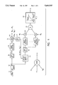
Referring now to the drawings in detail, and more particularly to FIG. 1, the reference character 11 represents a scene that is captured by image sensor 12. Image sensor 12 may be an electronic camera, video camera, laser, etc. The output of sensor 12 is an analog signal (V_i), that is coupled to analog to digital converter 14. Analog to digital converter 14 digitizes the signal V_i to a raw gray scale image S_i which is stored in image buffer 15. Central processing unit 16 receives the raw digitized signal from buffers 15 and processes this signal in accordance with the enhancement algorithm to obtain a set of digital enhancement parameters (offsets P_i =(s_ai, s_bi) and weights (w_i)). The enhancement algorithm is hereinafter disclosed. The processed signal is converted to analog quantities by digital to analog converter 17. The digital enhancement parameters are P_i =(s_ai, s_bi) and the analog enhancement parameters are Q_i =(v_ai, v_bi). The aforementioned analog parameters Q_i are transmitted to offset block 13. Offset block 13 clips the analog signal V_i at the aforementioned signals high and low levels by offsets Q_i =(V_ai, v_bi). The clipped analog signal is transmitted to analog to digital converter 18. Analog to digital converter 18 digitizes the clipped analog signal and transmits L copies of the enhanced image T_i to the input of image buffers 19. There are L image buffers 19. In this embodiment L will be equal to three. Weight w_i is decomposed into a sum of L powers of two weights w_ij, j=1 . . . L. Image T_i is multiplied by weight w_ij by multiplier 20.

The output of multiplier 20 is connected to the input of summer 21. Summer 21 sums the multiplied enhanced image to produce an enhanced summed image of the scene at its output. The enhanced summed image of the scene may now be utilized for any purpose that is known in the art.

The output of summer 21 i.e. the enhanced summed image is passed through an activation function 22 illustrated by the graph to the right of summer 21. Any digitized gray scale value within S_min and S_max is passed as is. Any value exceeding S_max is truncated to S_max and any value below S_min is truncated to S_min.

The enhancing algorithm that is utilized by central processing unit 16 will be presented below in two steps:

Step 1

From a set of representative images, the model constants are estimated. This step is performed in an off-line process where the speed of the implementation is not critical. This step is usually performed once at the beginning of the experiment. However, the implementations presented in this invention are efficient and can be executed at high speeds.

Step 2

In this step, the enhanced image is generated from known model constants, and from user-specified desired gray values. The execution speed of this step is critical, since this step is performed repeatedly for every different image to be enhanced.

An algorithm to estimate model constants will be discussed hereinafter under the subheading Computation of Model Constants. A separate algorithm is discussed hereinafter under the subheading Estimation of Upper Limit g_max of gain g.

In our notations, we shall use upper case letters for images or vectors. Lower cases will be used for variable such as gray scale values or offsets. Although functions are defined for scalars, we shall use vectors as parameters for functions, where the functions are applied to each element of the vector.

Let Vε^N be an input analog image signal and Sε^N be a digitized ray gray scale image obtained by digitizing signal V to image S, where N is the number of digitized pixels. Note that input V can come from many sources such as sensors (cameras, lasers, etc.) or stored analog image signals. Within S, we shall identify M(1≦M≦N) disjoint non empty regions (R₁ . . . R_M) to be enhanced by our algorithm. Each Region R_i of S consists of a subset S_i .OR right.S of contiguous picture points. We shall define s_i as a measure for the set S_i, where s_i is the mean of S_i i=1 . . . M, although, in general, s_i can be any other measure such as the median, weighted average, standard deviation or random sample of the set S_i.

Let (s_min, s_max) be the complete range of the gray scale values in S. The permissible input range (v_min, v_max) is obtained by the transform h (see below) of (s_min, s_max), i.e. v_min =h(s_min) and v_max =h(s_max). Define θ={vε|v_min≦v≦v_max }, and Φ={sε|s_min ≦s≦s_max }.

The analog to digital converter (ADC) is a surjective map g:θ→Φ, where g^-1 does not exist. However, we shall define h:s|→v, where s is a gray scale value in image S and v is the mean of the analog values that are digitized to s. Thus h:Φ→θ is a bijective linear map. Also define V_i =h(S_i).

For every region R_i of S, the proposed algorithm allows the user to select a desired gray scale value d_i εΦ. Let U be the final enhanced image such that the mean gray scale value u_i for any region R_i within U equals d_i for i=1 . . . M.

For each region R_i of S we shall compute a set of digital parameters P_i =(s_ai, s_bi) and weight w_i. P_i includes a low offset s_ai, and a high offset s_bi which are transformed by the digital to analog converter (DAC)(h) to analog offsets Q_i =(v_ai, v_bi). Parameters Q_i are used to modify (offset) the input signal V_i by affine functions F_i ():θ→θ where ##EQU1##

The modified input F_i (V_i) is digitized by ADC to enhance image T_i. Image T_i is multiplied by weight w_i and passed through the activation function f() to obtain an enhanced image. Note that we have multiplied weight w_i to enhanced image T_i instead of inputs v_i or F_i (v_i). This is because most ADCs have the hardware to modify the input V_i but do not have a method of multiplying V_i by weight w_i. Approximating g to a linear function g, g(w_i F_i (V_i)) =w_i g(F_i (V_i))=w_i T_i. Therefore, multiplying F_i (V_i) by w_i is the same as multiplying T_i by w_i under this approximation.

In the proposed approach, our concern is to generate enhanced images from inputs V_i irrespective of their source. We shall, therefore, not use the actual measured value of input analog signal V_i or its modified value F_i (v_i). Instead, the raw gray scale image S and enhanced images T_i, are used in our computations.

In our application, we shall present an efficient implementation of the analytical models with an ADC. In the framework established above, the ADC performs two functions: (1) affine transformation F_i (), and (2) digitization g(). Note that although the analysis is carried out for the ADC, the general method described above can be applied to any hardware which conforms to functions F_i () and g() defined in our models.

Enhancement Model

We shall present an enhancement model to fit the non-idealities found in many common analog to digital converters (ADCs). Considering these non-idealities and ignoring second order error terms, we get the following expression for enhanced images T_i (see FIG. 1), where t_i εT_i :

t.sub.i =g.sub.i s.sub.i +k.sub.i g.sub.i s.sub.ai +k.sub.2 s.sub.ai +k.sub.3 s.sub.i +k.sub.4, i=1 . . . M, t.sub.i εΦ(1)

Here g_i is the gain: ##EQU2##

In (1), when s_ai =s_min, and s_bi =s_max we call it the full range operation. Output gray scale values s_i at full range are called the full range gray scale values. Note that s_i and t_i represent the ideal digitized values of v_i and F_i (v_i) respectively. The actual gray scale values are a round-off (quantization) of the ideal values.

Next the enhanced images U are obtained by the weighted sum of image T_i with weights w_i. Here {U_i, . . . U_M } form regions {R_i, . . . , R_M } respectively of the final enhanced image U. Thus, ##EQU3## As defined before, s_i is a mean (or any other measure) of the raw image S_i. Similarly t_i and u_i are the means (or any other measures) of enhanced images T_i and U_i respectively.

In (l), (k₁, k₂, k₃, k₄) are unknown real-valued model constants. The ideal values are: k₁ -1, k₂ =k₃ =0. k₄ represents any bias in the system. Ideally for an unbiased system, k₄ =s_min which is usually 0. It is clear from (1), that for unknown (k₁, k₂, k₃, k₄), the true values of s_i are unknown. Only the measured values m_i are obtained at full range operation as:

m.sub.i =(l+k.sub.3)s.sub.i +(k.sub.1 +k.sub.2) s.sub.min +k.sub.4, i=l . . . M                                                       (4)

We shall call m_i the measured full range gray scale values.

Perhaps it can be demonstrated that (1) can be derived by assuming non-idealities for other parameters or by assuming different non-idealities for the same parameters. However, our experiments show that (1), independent of its derivation, appropriately represents the non ideal system under discussion.

Computation of Model Constants

Before estimating (k₁, k₂, k₃, k₄) we should compute the upper limit g_max of gain g_i by the algorithm under the subheading estimation of upper limit g_max of Gain g and also identify M regions {R , . . . , R } for enhancement. From the estimate of g_max we obtain the following operating range for offsets (s_ai, s_bi) ( derived from (2)): ##EQU4## It is clear from (1) that the full range gray scale values s_i, i=l . . . M, are unknown variables in estimating constants (k₁, k₂, k₃, k₄). For this reason, we shall also estimate s_i along with model constants (k₁, k₂, k₃, k₄) as follows:

(1) For each region R_i, i=1 . . . M, choose K offsets (s_ak, s_bk), k=l . . . K, within constraint (5), and compute g_k by (2).

(2) For each (s_ak, s_bk) acquire an image and estimate t_ik by averaging gray scale values within R_i. Note that estimates of t_ik can be obtained by other methods such as choosing a median, or random sample of gray scale values within R_i. Eliminate those t_ik that are close to s_min and s_max.

(3) Equation (1) can be written in the following matrix form for each region R_i. ##EQU5## The above equation is solved by the least squares method. (4) Final estimates of (k₁, k₂) are obtained by averaging M estimates of (k₁, k₂) from M regions.

(5) From the M estimates of s_i and k₃ s_i +k₄, i=l . . . M, obtained above (6), we can estimate k₃ and k₄ by least squares method from the following equations: ##EQU6##

Experimental Results

The above algorithm for the estimation of model constants (k₁, k₂, k₃, k₄) is applied on a set of industrial samples of steel. Constants (k₁, k₂, k₃, k₄) estimated from 8 different parts are shown in Table 1 below:

              TABLE 1                                                     
______________________________________                                    
MODEL CONSTANTS (k.sub.1, k.sub.2, k.sub.3, k.sub.4) ESTIMATED FROM       
8 DIFFERENT PARTS                                                         
Samples   k.sub.1  k.sub.2    k.sub.3                                     
                                    k.sub.4                               
______________________________________                                    
1         -1.0480  -0.0270    0.590 -6.3590                               
2         -1.0284  -0.0106    0.0550                                      
                                    -6.0056                               
3         -1.0044  -0.0374    0.0550                                      
                                    -6.1488                               
4         -1.0210  -0.0210    0.0542                                      
                                    -5.9058                               
5         -1.0110  -0.0378    0.0582                                      
                                    -6.0118                               
6         -1.0300  -0.0108    0.0496                                      
                                    -5.6976                               
7         -1.0354  -0.0056    0.0564                                      
                                    -6.1598                               
8         -1.0196  -0.0244    0.0518                                      
                                    -5.2660                               
______________________________________

The table shows:

(1) Estimates of model constants (k₁, k₂, k₃) are close to their ideal values (ideal k₁ -1, k₂ =k₃ =0, k₄ =s_min =0).

(2) Estimate of bias constant k₄ is different from its ideal value of s_min =0. This result demonstrates that the ADC system has a bias that is represented by k₄, and the enhancement model (in (1)) has helped us arrive at accurate enhanced images, which can not be obtained without this model.

Estimation of Upper Limit g_max of ADC Gain g

In order to maintain the linearity assumptions made for (l), we should determine operating ranges of offsets s_a and s_b. For this reason, we shall first determine the range (g_min _g _max) for gain g. It is clear from (1) and (2) that the lower limit g_min of g is obtained for the full range operation (i.e. s_a=s _min, s_b =s_max) where g=1.

Before determining the upper limit g_max of g, we should establish the experimental conditions to acquire valid data to properly estimate g_max. Since setting offsets (s_a, s_b) decreases the dynamic range of input V, we should make sure that V is well distributed within θ=[v_min, v_max ] for g=1. If input is distributed close to limits v_min or v_max for g=1, setting offsets (V_a, V_b) will further limit V, and reduce the availability of reliable data for accurate estimation of g_max. An easy way to check this condition, is to acquire an image S, and measure gray scale values at different regions of interest within the image. If these gray scale values are distributed close to s_min or s_max, the optical setup conditions such as lens aperture and illumination should be reconfigured so that they are within (s_min, s_max).

Estimate g_max by the following steps:

1. Place a part under the camera with the optical condition established above.

2. Select M (M≧2) regions of interest {R₁, . . . R_M } within the image.

3. Start from the first region R₁, i.e. R_i =R₁, where index i is the i^th estimate of g_max from region R₁.

4. Assuming a "reasonable" value g_start ≧1 of g_max (say g_start =1.5), estimate model constants (k₁, k₂, k₃, k₄).

5. Choose a set of K offsets (s_ak, s_bk), k=1 . . . K, within constraint (5).

6. For each choice of offset (s_ak, s_bk), k=1 . . . K, perform the following steps:

6.1 Acquire an image with offsets (s_ak, s_bk).

6.2 From this acquired image measure gray scale value t_ik.sbsb.--_measured by averaging gray scale values within region R_i. Eliminate values that are close to s_min and s_max.

6.3 Compute gray scale value t_ik.sbsb.--_computed from (1).

6.4 Compute the error (e_k) between the measured and computed gray scale values i.e. e_k =t_ik.sbsb.--_measured t_ik.sbsb.--_computed.

6.5 compute gain g_k from (2).

7. Choosing a limit e_max of error e_k k=1 . . . K, estimate the upper limit g_max ^R.sbsp.1 of gain g from region R₁.

8. If g_max ^R.sbsp.1 <g_max then set g_start =g_max ^R.sbsp.i and repeat steps 4-7 till g_max ^R.sbsp.1 ≧g_start.

9. If g_max ^R.sbsp.i ≧g_start, then report g_max ^R.sbsp.i as the estimate of g_max from region R_i.

10. Repeat steps 5-9 for all selected regions R₁, . . . , R_M.

11. Choose the final estimate g_max as the minimum value of all estimates: g_max =min {g_max ^R.sbsp.i, i=l . . . M}.

Appropriate Selection of M Regions {R₁, . . . , R_M }.

Here we shall first partition the image into M disjoint non empty regions of interest {R₁, . . . , R_M }. The M regions are usually chosen by pre-defined criteria dependent on the application. For example, in an image with multiple parts on a background, each part and the background form regions {R₁, . . . R_M }. Instead of using the entire region R₁ for our computations, a small probing window within R₁ is chosen to reduce computational complexity.

Generation of Desired Enhanced Image

This analysis involves efficient estimation of offsets (s_ai, s_bi) and weights w_i, i=1 . . . M, from: (1) known model constants (k₁, k₂, k₃, k₄) , and (2) user-specified desired gray scale values (d₁, . . . , d_M) for regions {R₁, . . . , R_M } respectively. The enhanced gray scale image T_i is obtained by modifying input V_i by estimated offsets (s_ai, s_bi). The final enhanced image U_i =w_i T_i, where weights w_i are generated by our algorithm. From (1) and (3),

d.sub.i =w.sub.i (g.sub.i s.sub.i +k.sub.i g.sub.i s.sub.ai +k.sub.2 s.sub.ai +k.sub.3 s.sub.i +k.sub.4), i=1 . . . M, where d.sub.i εφ                                            (9)

We shall first determine a range R(s_ai) of low offset s_ai, R(g_i) of gain g_i and R(w_i) of weight w_i, such that when these parameters are within their respective ranges, we shall obtain enhanced gray scale values t_i εΦ where t_i εT_i.R(s_ai) is shown below (derived from (5) and t_i εΦ in (1)): ##EQU7## A plot of s_ai against different values of g_i is shown in FIG. 3 for s_i =100 (FIG. 3A) and s_i =200 (FIG. 3B).

In (2) we can choose (s_ai, s_bi) such that 1<g_i <s_max -s_min. However, the linearity assumptions of ADC(g) in (1) are invalid for g_i >g_max (g_max<s _max-s _min) where g_max is determined experimentally. We, therefore, have the following permissible range R(g_i) for gain g_i.

R(g.sub.i):1≦g.sub.i ≦g.sub.max              (11)

It is clear from (9) that given any (g_i, s_ai) we can obtain the desired d_i by adjusting weight w_i. It is therefore, not so interesting to study the solution to (9) for any arbitrary weight w_i. Since there can be several choices of w_i ≦0, the optimum choice may be determined from computational considerations. The best choice is 1, which requires no more processing than a simple image acquisition. In one example, it took us 144 seconds to multiply an entire image (512×480 pixel resolution) with a weight, whereas it took, us 33 ms to acquire an image. If w_i =1 is not a valid solution for (9), choose w_i closest to 1. Multiplying by w_i >1(w_i <1) may raise (lower) some gray values above (below) s_max (s_min) which are truncated to s_max (s_min) by activation function f() in FIG. 1. Choosing w_i closest to 1 minimizes this loss of accuracy due to truncation. We shall, therefore, solve (9) for w_i closest to 1. An efficient method of multiplying enhanced image T_i with w_i ≠1 is discussed herein.

Compute (g_i, s_ai) by the following algorithm:

(1) Choose the starting value of w_i =1.

(2) Choose the starting value of g_i =1.

(3) Check if s_ai satisfies the following inequality (obtained from (9) and (10)): ##EQU8## (4) If s_ai does not satisfy (12), increment g_i (by say 0.1) and go back to step 3.

(5) If s_ai satisfies (12), report g_i, s_ai and w_i and terminate the algorithm.

(6) Continue the search till g_i =g_max. If g_max does not satisfy (12) check the following:

(6.1) If s_ai computed from (12) with g_i =g_max exceeds the upper limit in R(s_ai) then increment w_i by 2^-L where L is determined in a later section.

(6.2) If s_ai computed from (12) with g_i =g_max is below the lower limit in R(s_ai) then decrement w_i by 2^-L.

(6.3) Go back to step 2.

Note that the algorithm chooses the smallest permissible value of g_i, because the linearity assumption of the ADC is strongest for g_i closest to 1. Parameter s_bi is obtained as ##EQU9##

Permissible Range of Desired Gray Scale Values d_i, i=1 . . . M

Here we shall study a range R(d_i) of desired gray scale values d_i, so that when d_i are chosen within R(d_i), we can obtain an enhanced image by our algorithm. As seen before, we can obtain any value of d_i by appropriately adjusting values of weight w_i. It is, therefore, not so interesting to study the model for any arbitrary weight w_i. It is, however, important to obtain the desired gray scale value d_i with w_i =1 in order to reduce computation.

If we select d_i .epsilon slash.R(d_i), we have three choices:

(1) We can choose a weight w_i such that d_i can be obtained. This is the less preferable option due to computational considerations.

(2) From a plot of R(d_i) choose "satisfactory" values of d_i within it.

(3) Obtain guidelines to change the optical/illumination setup to attain d_i with our algorithm.

Assuming (k₁, k₂, k₃, k₄) close to their ideal values, we obtain: ##EQU10## For the ideal case, the above equation can be simplified to the following: ##EQU11## A plot of R (d_i) for this case is shown in FIG. 5. Here we observe that for s_i =100, we can obtain all values of d_i with our algorithm. For s_i =200, we can only obtain higher values of d_i >123. Thus, low values of s_i gives us greater choices of d_i.

If our choice of d_i .epsilon slash.R(d_i), we need to reconfigure the imaging conditions (such as by adjusting the camera-lens or illumination setup) so that d_i εR(d_i). In (13), R(d_i) depends on s_i and we observed in FIG. 5 that appropriate choices of s_i gives us wider choices of d_i. We, therefore, need to find a range R(s_i) for s_i such that if s_i εR(s_i) then d_i can be obtained with our algorithm. Assuming (k₁, k₂, k₃, k₄) close to their ideal values: ##EQU12## A plot of s_i against different values of g_i and s_ai is shown in FIG. 6. To change the imaging conditions, the camera-lens and illumination setup are reconfigured so that s_i εR(s_i).

Weighted Sum of L Enhanced Images

Among the computations involved in the algorithms described above, it is the multiplication by weight w_i that makes it difficult to implement the method with digital hardware. If w_i =1 is not a feasible choice, we have the following disadvantages:

1. It is usually computationally inefficient to multiply an entire image with a number.

2. Multiplication with any number, especially noninteger numbers, can cause loss of gray scale value information due to roundoff or truncation.

In most image processors it is simpler to add or subtract images than to multiply an image with a number. In one example, we added/subtracted two images (512×480 pixel resolution) in 10 ms, while it took us 144 s to multiply the image with a number.

One possible way to solve this problem is to use powers-of-two weights such that the multipliers are replaced by shift registers. This means that the weights can only take values on {0, 1, ±2^-1, ±2^-2, . . . ±2^-L }, where L is determined by the accuracy required. Thus ##EQU13## where w_ij are powers-of-two weights. Multiplication of image T_i by weight w_ij =2^-k is realized by left shift of every pixel value by k steps. Clearly, any choice of L gives us an accuracy ≧2^-L. Furthermore, L can be chosen from the number of bits used to store each gray scale value. For 256 gray scale values (represented by 8 bits) L can be chosen as 7, and the smallest weight change in step 6 of the enhancement algorithm is 2^-7. This method has the following advantages:

1. We may be able to choose w_ij =1 which may be otherwise impossible, and thus reduce computation.

2. Adding/subtracting images with w_ij =1 causes no loss of information due to round off errors.

3. Adding/subtracting images has the added benefit of noise reduction due to averaging of the noise. The improvement in image quality (signal-to-noise ratio) is proportional to the square root of L.

Simplified Enhancement Model

In this section we shall consider a simplification of the enhancement model described above. Instead of parameters P_i =(s_ai, s_bi) for individual regions, we shall apply the same parameter set P=(s_a, s_b) and weight w for all regions R_i, i=1 . . . M of the image. The advantages are:

(1) This model is computational efficient, and can be optimized to execute at real-time speeds.

(2) The model allows us to compute a single set of parameters P=(s_a, s_b) and weight w for the entire image.

(3) Since the parameters are the same over the entire image, we do not need any information on the boundaries of regions {R₁, . . . , R_M }, to be enhanced.

The new model is:

t.sub.i =gs.sub.i +k.sub.1 gs.sub.a +k.sub.2 s.sub.a +k.sub.3 s.sub.i +k.sub.4, and u.sub.i =f(wt.sub.i), and t.sub.i εφ, i=1 . . . M(16)

Generation of Enhanced Image from Known Model Constants

Here we shall estimate offsets (s_a, s_b) and weight w from: (1) known model constants (k₁, k₂, k₃, k₄) and (2) user-specified desired gray scale values d_i for regions R_i, i=1 . . . M. The enhanced image T is obtained by modifying input V by estimated offsets (s_a, s_b). The final enhanced image U=wT. From(16),

d.sub.i =w(gs.sub.i +k.sub.1 gs.sub.a +k.sub.2 s.sub.a +k.sub.3 s.sub.i +k.sub.4), whered.sub.i εφ, i=1 . . . M       (17)

From (17), (g and s_a are unknown), we obtain the following linear equation: ##EQU14## Since (18) is an overdetermined system, the following theorem describes the conditions on d_i, i=1 . . . M, under which solutions for g, s_a and w exist.

Theorem

From (18) the necessary and sufficient condition for which solutions for g, s_a and w exist is: ##EQU15##

for all i, j, k, l=1, . . . , M such that i≠j and k≠l(19)

Proof

For any pair of equations indexed by i and j, the solutions to (18) are: ##EQU16## If (18) has a solution then α_ij =α_k and β_ij=β_k. Considering only α_ij and α_kl we get (19). Next we shall show that if (19) is true, then (18) has a solution. In other words, we have to show that β_ij =β_kl and α_ij =β_kl if (19) is true. Clearly, from (19) and (19a) α_ij =α_kl. From (19a) ##EQU17## From this we conclude: β_ij -β_kl =0. Therefore, β_ij =β_kl. Q.E.D.

Theorem 1 shows that we can only choose two independent values of d_i for a single image, the rest of which are fixed by (19). Since we have only two offsets (s_a, s_b), to modify input V (giving us only two degrees of freedom), we can independently choose only two regions for simultaneous enhancement, i.e. M=2. Thus, we shall consider only two regions i and j for enhancement, for the rest of this analysis.

Next, we need to determine a range of (w, g, s_a) such that t_i εΦ when (w, g, s_a) belong to their respective ranges. Assuming s_i >s_j, without loss of generality, the range R(s_a) for s_a is (from (10)): ##EQU18##

R(g) for gain g is: R(g): 1≦g≦g.sub.max      (21)

For the nonideal case, we shall first determine a range R(w) for weight w such that when wεR(w), (g, s_a) satisfy (21) and (20) respectively. From R(g) in (21), we get the range R₁ (w): ##EQU19## From R(s_a) in (20) we get the range R₂ (w): ##EQU20##

The final range R(w) is: R(w)=R.sub.1 (w)∩R.sub.2 (w).(24)

The algorithm for enhancement is as follows:

1. Choose wεR(w). As before the best selection of w is 1. Otherwise choose w closest to 1 to minimize truncation and round-off errors due to activation function f() in FIG. 1.

2. Compute (g, s_a) from (18) satisfying (21) and (20) respectively.

3. Compute high offset S_b from: ##EQU21##

Second Order Measures of Desired Gray Scale Values

In all our previous discussions we have only considered the first ordered measures of the desired gray scale values d_i. These measures include the mean, median, weighted average and the random sample of d_i. All these measures of d_i follow a linear equation in (1). In this section, we shall discuss a second order measure of d_i. This measure is the standard deviation σ(d_i) of d_i. From (1) we obtain: σ(d_i)=w_i (g_i +k₃)σ(s_i), where σ(s_i) is the standard deviation of full range gray scale values s_i in raw image S_i.

If we need to enhance the image such that both first and second order measures need to be satisfied, we can modify step 2 of the enhancement algorithm such that g_i =1 is replaced by ##EQU22## The rest of the algorithm remains the same. Other second order measures that can also be considered by the above methods are a variation of gray scale values or a range of intensities about the mean.

FIG. 2 is a drawing that shows the result of an experiment which demonstrates a typical profile or error in gray scale values vs. gain that is used to estimate g_max by the algorithm hereinbefore stated.

Choosing a maximum error of 2 gray scale values, we estimated g_max =2.2 from FIG. 2. It is clear from FIG. 2, that the errors increase significantly for g>2.2. The range of offsets s_a and s_b determined from (5) is: (s_a +116)≦s_b.

FIG. 3A is a graph showing a range R(s_a) of low offset s_ai for different values of ADC gain for full range gray scale value s_i =100. The lower and upper curves are the lower and upper limits of the low offset s_ai.

FIG. 3B is a graph showing a range R(s_ai) of low offsets s_ai for different values of ADC gains g_i for full range gray scale values S_i =200. The lower and upper curves are the lower and upper limits of the low offset s_ai.

FIG. 4A is a drawing of two industrial steel samples with laser etched characters on them. The figure also shows the difference in contrast between the two parts.

FIG. 4B is a drawing of some characters in each part enhanced by the enhancement model and segmented by a standard segmentation algorithm. FIG. 4B also shows that characters not enhanced by the model are not clearly segmented;

FIG. 5A is a drawing of desired gray scale values d_i that can be obtained for different values of low offsets _ai and ADC gain g_i for full range gray scale value s_i =100. The figure also shows that all desired gray scale values can be obtained with our model in this case, for weight w_i =1.

FIG. 5B is a drawing of desired gray scale values d_i that can be obtained for different values of low offset s_ai and ADC gain g_i for full range gray scale value s_i =200. The figure also shows that only desired gray scale values >123 can be obtained with our model in this case, for weight w_i =1;

The above specification describes new and improved image enhancement system for visual recognition systems. It is realized that the above description may indicate to those skilled in the art additional ways in which the principles of this invention may be used without departing from the spirit. It is, therefore, intended that this invention be limited only by the scope of the appended claims.

Claims

What is claimed is:

1. An image enhancement system that enhances images, said system comprising:

means for capturing an analog image signal V of a scene;

first means coupled to said capturing means for digitizing the image to a raw gray scale image S;

means coupled to said digitizing means for processing the raw gray scale image S in accordance with

t.sub.i =gs.sub.i +k.sub.1 gs.sub.a +k.sub.2 s.sub.a +k.sub.3 s.sub.i +k.sub.4, i=1 . . . M

where t_i is a gray scale value, g is a gain, S_a is a low offset, S_i is a full range gray scale value, k₁, k₂, k₃, k₄ are constants, and M is a maximum number of regions to be enhanced,

to obtain a set of digital enhancement offset parameters P and weights w to produce a processed signal;

means coupled to said processing means for converting the digital enhancement parameters P into analog enhancement parameters Q;

means coupled to said capturing means and said converting means for stretching and clipping the analog signal V by analog enhancement parameters Q;

second means coupled to said stretching and clipping means for digitizing the stretched and clipped analog signal V to produce an enhanced image T;

means coupled to said second means for multiplying said enhanced image T by a multiplying weight w; and

means coupled to said multiplying weight w and to said enhanced image signal T for producing an enhanced final image U of the scene.

2. An image enhancement system that enhances images, said system comprising:

means for capturing an analog image signal V_i of a scene;

first means coupled to said capturing means for digitizing the image to a raw gray scale image S_i ;

means coupled to said digitizing means for processing the raw gray scale image S_i in accordance with

t.sub.i =g.sub.i s.sub.i +k.sub.1 g.sub.i s.sub.ai +k.sub.2 s.sub.ai +k.sub.3 s.sub.i +k.sub.4, i=1 . . . M

where t_i is a gray scale value, g_i is a gain, S_ai is a low offset, S_i is a full range gray scale value, k₁, k₂, k₃, k₄ are constants, and M is a maximum number of regions to be enhanced,

to obtain a set of digital enhancement offset parameters P_i and weights w_i ;

means coupled to said processing means for converting the digital enhancement parameters P_i into analog enhancement parameters Q_i ;

means coupled to said capturing means and said converting means for stretching and clipping the analog signal V_i by analog enhancement parameters Q_i ;

second means coupled to said stretching and clipping means for digitizing the stretched and clipped analog signal V_i to produce an enhanced image signal T_i ;

means coupled to said second means for multiplying weight w_i to enhanced image signal T_i ;

means coupled to said multiplying means for changing the multiplied enhanced image by activation function f() to produce an enhanced image U_i of the scene; and

means coupled to said changing means for combining enhanced images U_i to generate a final enhanced image U.

3. The system claimed in claim 2, further including first buffering means whose input is coupled to said first digitizing means and whose output is coupled to said processing means for buffering the input to said processing means.

4. The system claimed in claim 1, further including second buffering means whose input is coupled to said second digitizing means and whose output is coupled to said multiplying means for buffering the input to said multiplying means.

5. The system claimed in claim 2, wherein said capturing means is comprised of an electronic camera.

6. The system claimed in claim 2, wherein said capturing means is comprised of a video camera.

7. The system claimed in claim 2, wherein said capturing means is comprised of a laser.

8. The system claimed in claim 2, further including means for producing L copies of an enhanced image T_i.

9. The system claimed in claim 8, wherein said means for producing L copies comprises:

means for decomposing weight w_i into a sum of L powers of two weights, w_ij ;

means for multiplying image T_i with each weight w_ij ; and

means for summing the L weighted images.

10. The system claimed in claim 2, further including means for creating a desired gray scale value distribution in each region by varying w_i.

11. The system claimed in claim 10, further including means for changing a range of gray scale values.

12. The system claimed in claim 2, further including means for adjusting an illumination of the image.

13. The system claimed in claim 2, further including:

first means for selecting statistical measures of desired gray scale values in the enhanced image;

second means for selecting first order statistical measures such as mean, median, weighted average, or random sample and;

third means for selecting to second order statistical measures such as variance, variation, or range of intensities about the mean.

14. A method of producing an enhanced image, said method comprising the steps of:

capturing an analog image signal V_i of a scene;

digitizing the captured image signal to a raw gray scale image S_i ;

processing the raw gray scale image S_i in accordance with

t.sub.i =g.sub.i s.sub.i +k.sub.1 g.sub.i s.sub.ai +k.sub.2 s.sub.ai +k.sub.3 s.sub.i +k.sub.4, i=1 . . . M,

to obtain a set of enhanced parameter offsets P_i and weights W_i to produce a processed signal;

converting the processed signal into an analog signal that has analog enhancement parameters Q₁ by applying a transform function to V_i to both stretch and clip V_i ;

digitizing the transformed analog signal V_i to produce L copies of an enhanced image signal T_i ;

multiplying weight w_i to enhanced image signal T_i ;

changing the multiplied enhanced image by activation function f() to produce an enhanced image U_i of the scene; and

combining the enhanced image U_i to generate final enhanced image U.

15. An image enhancement system that enhances images, said system comprising:

means for capturing an analog image signal V_i of a scene;

first means coupled to said capturing means for digitizing the analog signal V_i to a raw gray scale image S_i ;

means coupled to said digitizing means for processing the raw gray scale image S_i in accordance with an enhancement algorithm to obtain a set of digital enhancement parameters P_i =(s_ai, s_bi), and weights w_i ;

means of obtaining a separate set of enhancement parameters P_i =(s_ai, s_bi), and weights w_i for each region i of the image;

means coupled to said processing means for converting said digital enhancement parameters into analog enhancement parameters Q_i =(v_ai, v_bi);

means coupled to said capturing means and said converting means for stretching and clipping the analog image signal V_i in accordance with ##EQU23## where V_i is clipped at its low and high levels v_ai and v_bi respectively by analog enhancement parameters Q_i =(v_ai, v_bi);

second means coupled to said stretching and clipping means for digitizing the stretched and clipped analog signal V_i to produce an enhanced gray scale image T_i ;

means coupled to said second means for multiplying the enhanced gray scale image T_i with weights w_i to produce a multiplied enhanced image W_i T_i ;

means coupled to said multiplying means for clipping the said multiplied enhanced image with the activation function f() in accordance with ##EQU24## to produce a final enhanced image U_i and; means coupled to said clipping means for combining enhanced images U_i in accordance with ##EQU25## to generate a final enhanced image U.

16. The system claimed in claim 14, further including:

means for producing L copies of an enhanced image T_i.

17. The system claimed in claim 15, further including

means of selection M regions for enhancement;

means of applying the enhancement algorithm on each of the said regions to obtain an enhanced image U_i ;

means of combining enhanced images U_i for each region to obtain final enhanced image U in accordance with ##EQU26##

18. The image enhancement system claimed in claim 14, further including:

means for determining the lower and upper bounds of first and second order measures of desired gray scale values and;

means for selecting measures of desired gray scale values within the said bounds to obtain the desired enhanced gray scale image.

19. The image enhancement system claimed in claim 14 further including:

means for determining a feedback to the system in order to obtain a desired enhancement.

20. An image enhancement system that enhances images, said system comprising:

means for capturing an analog image signal V_i of a scene;

means coupled to said digitizing means for processing the raw gray scale image S_i in accordance with ##EQU27## where d_i is a desired gray scale value for region i, k₁, k₂, k₃, k₄ are constants, g is a gain, and M is a maximum number of regions to be enhanced,

to obtain a set of digital enhancement parameters P=(s_a, s_b) and weight w;

means for obtaining said enhancement parameters P=(s_a, s_b), and weight w for all regions of the image;

means coupled to said processing means for converting said digital enhancement parameters into analog enhancement parameters Q=(v_a, v_b);

means coupled to said capturing means and said converting means for stretching and clipping the analog image signal V_i in accordance with a transform function F_i : ##EQU28## the analog image signal being clipped at its low and high levels v_a and v_b respectively;

second means coupled to said stretching and clipping means for digitizing the stretched and clipped analog signal V_i to produce an enhanced gray scale image T;

means coupled to said second means for multiplying the enhanced gray scale image T with weight w to produce a multiplied enhanced image and;

means coupled to said multiplying means for transforming the said multiplied enhanced image with an activation function f() in accordance with ##EQU29## to produce a final enhanced image U.

21. The system claimed in claim 20 wherein said system operates to enhance images to desired measures of gray scale values in real-time speeds.